The Question Everyone Is Asking (But Few Define Clearly)
“Can large language models think?” has become a shorthand for a deeper and more nuanced question: are these systems capable of generating genuinely original ideas, or are they merely sophisticated remix engines? The distinction matters - not just philosophically, but practically for how we evaluate research, deploy systems, and interpret outputs in high-stakes domains.
The conversation often collapses into extremes. On one side, LLMs are framed as stochastic parrots. On the other, they are portrayed as emerging minds. Neither position survives careful technical scrutiny.
To move forward, we need to define original thought in operational terms and evaluate LLMs against measurable criteria rather than intuition.
Defining “Original Thought” in Computational Terms
In human cognition, originality is typically associated with novelty, usefulness, and non-obviousness. Translating that into machine learning, we can decompose originality into three measurable signals:
Statistical Novelty: Outputs that are not memorized or trivially reconstructed from training data
Compositional Generalization: The ability to combine known concepts into previously unseen structures
Goal-Directed Synthesis: Producing ideas that satisfy constraints not explicitly present during training
Recent work in transformer-based architectures suggests that LLMs perform strongly in the second category, moderately in the third, and ambiguously in the first.
This already hints at a conclusion: LLMs are not simply copying - but they are also not independently “thinking” in the human sense.
What the Research Actually Shows
Empirical studies over the past two years have shifted the tone of this debate. Benchmarks such as BIG-bench, MMLU, and GSM8K demonstrate that models can solve tasks requiring multi-step reasoning and abstraction. However, deeper analysis reveals something more subtle.
A 2023–2025 line of research into mechanistic interpretability shows that LLMs rely heavily on pattern superposition rather than symbolic reasoning. In other words, they interpolate across dense statistical manifolds instead of constructing ideas from first principles.
Yet, in controlled experiments involving creative synthesis tasks - such as generating novel scientific hypotheses or designing algorithms - models have produced outputs that human evaluators rate as “original.” The catch is that these outputs often emerge from recombination at scale rather than intentional insight.
This leads to a critical reframing: originality in LLMs may be an emergent property of scale and diversity, not cognition.
A Practical Framework for Evaluating LLM Creativity
To move beyond vague claims, I’ve been using a four-layer evaluation framework in production systems to assess whether an LLM output crosses the threshold into meaningful originality.
Layer 1: Data Traceability
Can the output be linked back to known training examples via similarity search or embedding overlap?
Layer 2: Structural Novelty
Does the output introduce a new structure, method, or combination not seen in benchmark datasets?
Layer 3: Constraint Satisfaction
Can the model generate solutions under constraints that were never jointly represented during training?
Layer 4: Iterative Refinement Capacity
Does the model improve its own idea through self-critique loops?
In internal evaluations, most LLM outputs fail at Layer 1 when rigorously tested, pass Layer 2 inconsistently, and perform surprisingly well at Layer 4 when paired with tool-use or agent frameworks.
This suggests that creativity is not a static property of the model - but a system-level behavior.
Where LLMs Actually Excel: Combinatorial Creativity
If we examine outputs that appear “creative,” a consistent pattern emerges. LLMs excel at:
Cross-domain synthesis
Analogical reasoning
Style transfer across conceptual spaces
For example, when prompted to design a new distributed systems protocol inspired by biological processes, models often generate plausible hybrid designs that are not directly traceable to canonical papers.
However, when evaluated rigorously, these ideas tend to fall into what we might call bounded originality - novel within a constrained conceptual neighborhood.
This is not trivial. In many engineering contexts, bounded originality is exactly what we need.
Failure Modes: Where the Illusion Breaks
Despite impressive outputs, there are clear and repeatable failure modes that expose the limits of LLM creativity.
One major issue is semantic drift under novelty pressure. When pushed to be highly original, models often produce internally inconsistent or physically impossible ideas.
Another is false abstraction, where the model generates language that sounds conceptually deep but collapses under formal analysis.
In experimental settings, I’ve observed that introducing adversarial constraints - such as requiring proofs, edge-case handling, or computational validation - causes many “creative” outputs to degrade rapidly.
This reinforces the idea that LLMs lack grounded understanding, even when they produce convincing abstractions.
A Minimal Architecture for Enhancing Machine Creativity
Pure LLMs are not the endpoint. Systems that exhibit stronger forms of creativity tend to include additional components.
A simple architecture that has shown promising results in my own experiments includes:
When combined with external tools such as symbolic solvers or simulators, this loop significantly increases the rate of outputs that pass higher layers of originality.
This again points to a key insight: creativity emerges from interaction, not isolation.
Trade-offs: Originality vs Reliability
There is a fundamental tension between creativity and correctness in LLM systems.
As temperature and sampling diversity increase, outputs become more novel - but also less reliable. Conversely, deterministic decoding improves factual accuracy while suppressing creative variation.
In production environments, this trade-off must be explicitly managed. One effective strategy is to separate generation and validation phases, allowing the system to explore broadly before filtering aggressively.
This mirrors human creative processes more closely than single-pass generation.
So, Are LLMs Capable of Original Thought?
The answer depends on how strictly you define “thought.”
If originality requires intentionality, self-awareness, and grounded reasoning, then LLMs do not qualify.
But if we define originality as the ability to generate novel, useful, and non-trivial ideas through compositional processes, then the answer is more nuanced:
LLMs exhibit a form of emergent, system-level originality - without possessing true independent thought.
This distinction is not just philosophical. It has direct implications for how we design systems, evaluate contributions, and attribute credit in AI-assisted work.
The Real Shift Most People Miss
The most important takeaway isn’t whether LLMs think.
It’s that the unit of creativity is no longer the model - it’s the pipeline.
Engineers who understand this are already moving beyond prompt engineering into system design: building architectures where models, tools, memory, and evaluation loops interact to produce outputs that look increasingly like original contributions.
That’s where the real frontier is.
And that’s where the conversation should be.
After two years of bouncing between Claude desktop, ChatGPT voice, Gemini, and a half-dozen Ollama frontends, I got tired of the wake-word thrash. Every assistant assumes you’ve picked their team forever.
So I built BRAGI — a voice layer that runs locally, listens locally, and routes to whichever AI I tell it to. Including the one running on the same machine.
This post is the architecture, not a sales pitch. If you’ve been thinking about building something similar, here’s what I learned shipping v0.2.
The pipeline
Mic input
↓
openwakeword (local) — “Hey Jarvis”
↓
faster-whisper medium (local, GPU optional)
↓
Provider router (settings UI picks destination)
↓
[Cloud: Claude / OpenAI / Gemini / Grok / Groq / Together / HuggingFace]
[Local: Ollama / LM Studio / FREYA / Echo]
↓
TTS (eSpeak free, OpenAI Nova BYOK)
↓
Speaker output
Audio never leaves the machine. Only transcribed text goes to whichever cloud you picked, if any.
Wake word
openwakeword is the right call for a sovereign product. Picovoice is better quality but locks you into a paid commercial license. openwakeword is Apache 2.0 and runs on CPU.
The catch: training your own custom model requires matching the feature dimensions to whichever preprocessor version you’re targeting. I burned half a day on a model that had 96×103 features when openwakeword expected 32×147. v0.2 ships with the stock “Hey Jarvis” model and includes the custom “Hey BRAGI” model for users with compatible hardware.
STT
faster-whisper medium on CUDA is the sweet spot. Tiny is too inaccurate for real conversation, large is overkill for short voice commands. Medium gets ~1 second latency on a midrange GPU and handles bilingual input out of the box.
Critical detail: instantiate Whisper once at startup, never per-request. First inference call takes 5-10 seconds to warm CUDA. Users won’t tolerate that on every wake.
The router
This was the hardest part. Each provider has a different SDK, different streaming format, different auth pattern. The router abstracts that into one interface:
Each provider implementation handles its own SDK quirks. The router just picks one based on user settings or voice command (“BRAGI, switch to Claude”) and calls respond().
For local models I support both Ollama (HTTP API) and LM Studio (OpenAI-compatible HTTP API). Both run on the user’s machine. Both look identical to the router.
TTS
eSpeak ships with the installer because it’s free, offline, and 100+ languages. It sounds robotic. That’s fine. People who want premium voice can paste an OpenAI API key and use Nova.
I tried Kokoro for higher-quality offline TTS. Worked great in dev. Production builds kept hitting a 404 on the default voice file in HuggingFace. Shipped with eSpeak as the default and Kokoro as best-effort.
The settings UI
Local web UI on http://127.0.0.1:7777. Configure providers, paste API keys, pick voices, manage license. Page lives on the user’s machine. No account, no login, no cloud dashboard.
API keys live in a local vault. They never leave the machine. The product is sovereignty — that has to be true at every layer.
Stack
Python 3.11
openwakeword for wake detection
faster-whisper for STT
eSpeak / OpenAI Nova for TTS
FastAPI for the local settings server
pythonw.exe in tray mode for daily use
PyInstaller for bundling
NSIS for the Windows installer
~169MB installer, Win10/11
What I’d do differently
Custom wake word training is harder than the docs admit. openwakeword’s preprocessor is versioned and the feature dims have to match exactly. Document this for users who want to train their own.
PyInstaller + 4GB CUDA torch builds blow past NSIS’s 2GB single-file limit. I had to move torch + Kokoro to a first-run download instead of bundling them.
Don’t trust the embedded Python’s python311._pth defaults. User-site contamination from %APPDATA%RoamingPython will silently break your install. Always launch with -s -E flags.
What’s next
v0.3 will likely add: better Kokoro fallback, custom wake word training UI, multi-room concurrency. The architecture supports it — I just need to ship v0.2 first and see what users actually ask for.
If you want to see it: clintwave84.gumroad.com/l/leetkd
If you’ve built something similar and want to compare notes — drop a comment. Especially curious how others have handled the provider abstraction across cloud + local.
I’m Salah Eddine Medkour. I teach Python and ICT at Badji Mokhtar University in Annaba, Algeria, and I build things on the web when my brain won’t let me sleep. Before Nadeef, I made AirQuiz, an offline quiz platform that saved me 95% of my grading time when the university’s internet couldn’t handle 289 students taking exams simultaneously. I graduated with a master’s in Network Engineering, but most of what I actually build comes from being annoyed at problems that shouldn’t exist.
The trash pile that started everything
There’s a spot near my apartment. Trash bags piled against a crumbling concrete pillar under a highway overpass. It’s been there for three weeks. Every morning I walk past it. Every morning I think someone should clean it. Every morning I realize I’m “someone” and I keep walking.
This is the problem with civic responsibility. Everyone sees it. Nobody owns it. The municipality won’t come unless you call, and calling means navigating a phone tree that goes nowhere. Posting in a Facebook group gets 30 “inshallah someone fixes this” comments and zero action.
I wasn’t planning to build an app about this. I was scrolling through my Notes app looking for a grocery list when I found an entry from 2 AM three months ago. Just a title: “Trash reporting app but make it not annoying.” Below it, a messy diagram of pins on a map, some arrows, the word “gamification” circled twice.
I don’t remember writing this. But drunk-brain or sleep-deprived-brain or whatever version of me wrote it was right. The idea wouldn’t leave.
What Nadeef actually is
Nadeef means “clean” in Arabic. It’s a PWA, a progressive web app, which means it works on your phone without downloading anything from an app store. No 50MB install. No permissions popups. Just a link.
The concept is stupid simple. You see trash. You open Nadeef. You take a photo with your live camera (no uploading old photos from your gallery because people will absolutely try to cheat). GPS tags your exact location. You pick a severity level: minor litter, accumulated waste, or environmental hazard. You add a title. Done. A red pin drops on the map.
Someone else nearby sees the pin. They tap it. They see your photo, the location, how much XP they’ll earn for cleaning it. They accept the mission. They clean it. They take an after photo. You get a notification asking you to confirm the cleanup is real. You swipe through a before/after slider. If it looks good, you approve. They get XP. The pin turns green. Everyone moves on.
That’s the whole loop. Report, clean, verify, reward.
Why I built it in 24 hours
I gave myself one day. Not because I’m fast but because if I spend more than a weekend on something, I’ll overthink it into complexity and never ship.
I used what I knew would work: React for the UI, Supabase for the database and auth, Leaflet for maps, Netlify to host it. All free tiers. Zero dollars spent. I’m not trying to raise money or pitch investors. This is a tool, not a startup.
The tech stack matters less than the decisions I made while building:
Camera-only uploads. No gallery access. This prevents someone from uploading a photo they took six months ago and claiming they just cleaned a spot. The camera forces fresh photos with GPS metadata I can validate.
Before/after slider. This is the part I’m most proud of. It’s just two images with a draggable divider, but the emotional impact of sliding from dirty to clean is absurd. People spend 20 seconds just dragging the slider back and forth. It makes the transformation undeniable.
Gamification without manipulation. You earn XP for reporting and cleaning. You rank up from Scout to Pioneer to Guardian. You unlock badges for cleaning at dawn, cleaning in teams, being the first to clean in a new neighborhood. But there are no daily login streaks that punish you for missing a day. No dark patterns. No engineered addiction. Just visible progress for actual work.
Bilingual by default. The app is Arabic and English, toggled with one tap. Most civic tech ignores Arabic or treats it as an afterthought. I built the UI in both languages from day one, with proper right-to-left layout for Arabic, because half of Algeria prefers Arabic interfaces and they shouldn’t have to settle.
The philosophy underneath
Nadeef is not about altruism. It’s about ownership.
When trash sits on your street for weeks, you feel powerless. The system failed. The municipality didn’t come. Nobody cares. So you stop caring too. Learned helplessness.
Nadeef flips that. You see trash. You report it. Someone cleans it. You verify it. Suddenly you’re not powerless. You identified a problem. Someone else solved it. The system worked because you both made it work.
This is civic infrastructure built by civilians. No budget. No bureaucracy. Just people who live somewhere deciding that somewhere should be cleaner.
The gamification exists because humans are competitive and we respond to visible progress. The leaderboard shows you the top cleaners this week. The badges show you milestones. The XP number goes up. These are extrinsic motivators, sure, but they get people through the door. Once you’ve cleaned three spots and seen the before/after photos, you don’t need the XP anymore. You’re hooked on the transformation itself.
What people actually do with it
I seeded the app with 10 spots I cleaned myself. Trash under the highway. Litter near the university. A pile of branches blocking a sidewalk. I took before photos, cleaned them, took after photos, verified my own submissions at half XP (the system penalizes self-cleaning to prevent gaming).
Then I shared the link in a university WhatsApp group.
The first person to clean a spot I didn’t report was a master’s student named Yacine. He found a spot I had marked three days earlier. Bags of construction debris someone dumped near a school. He went there with two friends, filled the bags into a cart, hauled them to a dumpster, uploaded five photos showing the process.
When I got the notification to verify his cleanup, I dragged the before/after slider and felt something I wasn’t expecting. Pride. Not my pride. His. He took a problem I pointed at and he solved it. I just built the tool.
That’s when I knew this might work.
The problems I didn’t anticipate
Spam. Within 48 hours someone uploaded a photo of a cat and marked it as a level 3 environmental hazard. I added a flagging system.
Fake cleanups. Someone uploaded an after photo that was clearly just a different angle of the same trash pile. I tightened the EXIF validation and added community voting for suspicious submissions.
Territorial behavior. Two users started competing for the same spots. They’d both rush to claim a pin the second it appeared. I added a claim-locking system. Once someone hits “start cleaning,” they get a 30-minute exclusive window.
These are good problems. They mean people care enough to try to break the system.
What’s missing and what’s next
Nadeef has no business model. I’m not monetizing this. I’m not putting ads in it. I’m not selling data to waste management companies.
I do want partnerships, but only under specific terms. If a company wants to sponsor a cleanup campaign or fund supplies, fine. Any profit from those collaborations goes to registered charities or gets reinvested into cleanup campaigns. No one gets rich off people picking up trash.
I’m also terrible at promotion. The app exists. It works. I posted it on social media once. That’s the extent of my marketing. I’m open to volunteers who want to help spread it, moderate content, translate it to other languages, or build on top of it.
If an NGO in Tunisia or Morocco wants to adapt it for their city, the code will eventually be open source. Take it. Fork it. Make it better.
Right now I’m focused on making it work well in Annaba. Ten users cleaning three spots each per week is more valuable than 1,000 users who sign up, look around, and leave.
Why I’m writing this
I’m writing this because I want the app to show up when someone Googles “civic engagement Algeria” or “community cleanup tool” or “how to report trash in my city.”
I’m also writing this because building in public is uncomfortable and I need to get better at it. I don’t naturally share half-finished work. I don’t naturally ask for help. But Nadeef won’t scale if I’m the only one who knows it exists.
If you’re in Annaba and you’ve walked past the same trash pile for three weeks, try Nadeef. If you’re in another city and you want to adapt the idea, contact me. If you’re a graphic designer or developer or community organizer and you want to help, I’ll figure out how to coordinate volunteers.
The app is at nadeef.netlify.app. It’s a website. Open it on your phone. No download. No signup required to browse the map. You only need an account if you want to report or clean.
The source code isn’t public yet but it will be. React, Supabase, Leaflet, Tailwind. Standard modern web stack. Nothing fancy. It works.
The thing I keep thinking about
There’s a concept in Islam called sadaqah jariyah. Continuous charity. The idea is that some good deeds keep generating reward even after you die. Planting a tree. Digging a well. Teaching someone to read.
I’m not religious, but the concept resonates. If Nadeef helps someone clean one spot, and that inspires someone else to clean another, and that creates a norm where neighborhoods take care of themselves, then the initial effort compounds.
I didn’t set out to build something altruistic. I set out to scratch an itch. I was annoyed that trash sat in public spaces for weeks because the coordination problem was unsolved. So I solved the coordination problem.
If that happens to make the world slightly cleaner, I’ll take it. But mostly I just wanted to stop walking past that trash pile every morning and feeling helpless.
Now I don’t.
Salah Eddine Medkour is a web developer, network engineering graduate, and university instructor from Annaba, Algeria. He builds tools that solve problems he’s personally annoyed by. You can find him on LinkedIn or contact him at medkoursalaheddine@gmail.com.
My Website : salaheddinemedkour.me
Nadeef is live at NADEEF APP.
Last year, a deployment went sideways. An AI agent was running a data enrichment pipeline: pull records from an API, map fields into a schema, write to a database. Every API call returned 200 OK. The agent’s dashboard showed green across the board. The agent reported success on every step.
Six hours later, a downstream team flagged the data. Half the field mappings were hallucinated. The agent had confidently mapped company_revenue to employee_count, invented values for missing fields, and written duplicates for records it had already processed. Hundreds of bad rows, all marked as verified.
Nobody noticed because nothing “failed.”
This is the fundamental problem with AI agents in production: the most dangerous failures look exactly like success. Traditional error handling — try/catch blocks, HTTP status code checks, crash monitoring — was built for deterministic software. AI agents are probabilistic systems. They don’t crash when they’re wrong; they confidently produce garbage with a 200 status code.
After living through that incident and building dozens of production agents since, I’ve distilled five error handling patterns that actually work. Each pattern handles a failure mode the previous one can’t catch. Together, they form a defense-in-depth strategy that keeps agents running, prevents silent data corruption, and gives you sleep on weeknight deployments.
Pattern 1: Circuit Breakers for LLM Quality Failures (Not Just HTTP Errors)
The classic circuit breaker pattern — closed, open, half-open — is standard infrastructure engineering. But when it comes to AI agents, the traditional version is incomplete. It tracks HTTP failures. It misses quality failures.
The Problem
After a model provider degradation, an agent started returning malformed JSON. Every API call succeeded. The HTTP status was 200. We burned 40 minutes of compute before anyone noticed because nothing in the error handling checked output quality — only transport status.
The Solution: Quality-Aware Circuit BREAKER
A circuit breaker for agents needs to track quality failures: outputs that violate schema, fail semantic invariants, or produce unsafe actions — even when the API itself succeeds.
importtimefromenumimportEnumfromdataclassesimportdataclass,fieldclassCircuitState(Enum):CLOSED="closed"OPEN="open"HALF_OPEN="half_open"@dataclassclassQualityCircuitBreaker:failure_threshold:int=3reset_timeout:float=60.0state:CircuitState=CircuitState.CLOSEDfailures:int=0last_failure_time:float=field(default_factory=time.time)defrecord_quality_failure(self)->None:"""Called when LLM output fails validation (not HTTP error)."""self.failures+=1self.last_failure_time=time.time()ifself.failures>=self.failure_threshold:self.state=CircuitState.OPENdefrecord_success(self)->None:ifself.state==CircuitState.HALF_OPEN:self.state=CircuitState.CLOSEDself.failures=0defallow_request(self)->bool:ifself.state==CircuitState.CLOSED:returnTrueifself.state==CircuitState.OPEN:elapsed=time.time()-self.last_failure_timeifelapsed>=self.reset_timeout:self.state=CircuitState.HALF_OPENreturnTrue# One probe request
returnFalse# Circuit is open, reject
# Half-open: allow exactly one probe
returnTruedefshould_block(self)->bool:returnnotself.allow_request()
Key insight: When the circuit opens, stop. Don’t burn tokens on a model producing garbage. Wait for the cooldown, send one probe request, and if it passes schema validation, close the circuit.
A natural extension is a model fallback chain: when the circuit opens, switch to a cheaper model with tighter constraints (lower temperature, stricter schema, fewer allowed tools). Circuit breakers tell you when to stop trusting a model; fallback chains tell you where to go next.
Pattern 2: Validation Gates Before Tool Execution
An agent mapped a delete_all_records action to what it interpreted as “cleanup.” The API accepted it. 47 records gone before the next human review. The agent was confident. The action was syntactically valid. The intent was completely wrong.
The Rule
Never let an agent’s output directly trigger a side effect. Always validate before execution.
fromtypingimportAnyfromdataclassesimportdataclassimportjson@dataclassclassToolCallValidation:tool_name:strparameters:dict[str,Any]ALLOWED_TOOLS={"query_database","send_notification","update_record"}DESTRUCTIVE_TOOLS={"delete_record","archive_project"}MAX_DELETE_COUNT=10classValidationGate:defvalidate(self,call:ToolCallValidation)->tuple[bool,str]:"""Returns (is_valid, reason)"""# 1. Schema: is this a known tool?
ifcall.tool_namenotinALLOWED_TOOLS|DESTRUCTIVE_TOOLS:returnFalse,f"Unknown tool: {call.tool_name}"# 2. Sanity: does the action make sense?
ifcall.tool_name=="delete_record":count=call.parameters.get("count",1)ifcount>MAX_DELETE_COUNT:returnFalse,(f"Delete count {count} exceeds limit of {MAX_DELETE_COUNT}")# 3. Boundary: is the agent in its allowed scope?
ifcall.tool_name=="query_database":table=call.parameters.get("table")iftable=="production_billing":returnFalse,"Agent cannot access production_billing"returnTrue,"OK"
Three layers of validation, each catching a different failure class:
Schema validation — Is the output structurally correct? Missing required field? Wrong type? Malformed JSON?
Sanity checks — Does the action make sense? Deleting 10,000 records? Probably not.
Boundary enforcement — Is the agent operating within its allowed scope? Cross-tenant access? Targeting a production table from a staging workflow?
This gates every tool call before it executes. No separate validation function to remember to call — it’s in the critical path.
gate=ValidationGate()defexecute_tool_call(raw_llm_output:str):call=parse_tool_call(raw_llm_output)is_valid,reason=gate.validate(call)ifnotis_valid:logger.warning(f"Tool call blocked: {reason}")returnf"Action blocked: {reason}. Please revise."# Only reach here after validation passes
returnrun_actual_tool(call)
Design principle: Constrain what the agent can do, and you prevent most errors at the source. This pairs directly with the insight from tool design work — splitting one monolithic tool into eight focused tools eliminates most validation failures before they can occur.
Pattern 3: Idempotent Sagas for Multi-Step Workflows
A three-step agent workflow failed on step 2. Step 1 had already created a customer record. The retry created a duplicate. Two hundred orphaned records found a week later, each triggering duplicate billing notifications.
The math is uncomfortable: an agent that succeeds 95% of the time on each step has only a 60% chance of completing a 10-step workflow cleanly (0.95^10). At 90% per step, a 10-step workflow succeeds just 35% of the time. Every step compounds the risk, and without idempotency, every retry doubles the side effects.
The Solution: Checkpoint-Then-Execute with Compensation Actions
Borrowing from the saga pattern in distributed systems, each step records its completion before execution and defines a compensation action for rollback.
fromdataclassesimportdataclassfromenumimportEnumfromtypingimportCallable,Optionalimportsqlite3classStepStatus(Enum):PENDING="pending"COMPLETED="completed"COMPENSATED="compensated"@dataclassclassSagaStep:name:strexecute:Callablecompensate:Optional[Callable]# None means read-only or irreversible
status:StepStatus=StepStatus.PENDINGclassSagaExecutor:def__init__(self,db_path:str=":memory:"):self.conn=sqlite3.connect(db_path)self._init_checkpoint_table()def_init_checkpoint_table(self):self.conn.execute("""
CREATE TABLE IF NOT EXISTS checkpoints (
step_name TEXT PRIMARY KEY,
status TEXT,
result TEXT
)
""")self.conn.commit()def_is_completed(self,step_name:str)->bool:row=self.conn.execute("SELECT status FROM checkpoints WHERE step_name = ?",(step_name,)).fetchone()returnrowisnotNoneandrow[0]=="completed"def_record_checkpoint(self,step_name:str,result:str):self.conn.execute("INSERT OR REPLACE INTO checkpoints (step_name, status, result) ""VALUES (?, 'completed', ?)",(step_name,result))self.conn.commit()defexecute(self,steps:list[SagaStep])->dict[str,str]:completed_steps=[]forstepinsteps:ifself._is_completed(step.name):# Idempotent: skip already-completed steps on retry
continuetry:result=step.execute()self._record_checkpoint(step.name,str(result))completed_steps.append(step)exceptExceptionase:# Rollback: execute compensation in reverse order
logger.error(f"Step '{step.name}' failed: {e}. "f"Rolling back {len(completed_steps)} steps.")forcompletedinreversed(completed_steps):ifcompleted.compensate:try:completed.compensate()exceptExceptionascomp_err:logger.critical(f"Compensation for '{completed.name}' failed: "f"{comp_err}")raisereturn{s.name:"completed"forsinsteps}
Usage:
deffetch_data():returnapi.get_records()deftransform(data):return[process(r)forrindata]defwrite_to_db(data):db.insert_batch(data)return{"id":db.last_insert_id}defrollback_write(ctx):db.delete_batch(ctx["id"])defsend_notification():smtp.send("Pipeline complete")defsend_correction():smtp.send("Correction: pipeline was rolled back")saga=SagaExecutor()steps=[SagaStep("fetch_data",execute=fetch_data,compensate=None),# Read-only
SagaStep("transform",execute=transform,compensate=None),# Pure function
SagaStep("write_to_db",execute=write_to_db,compensate=rollback_write),SagaStep("send_notification",execute=send_notification,compensate=send_correction),]saga.execute(steps)
Classify every step:
Read-only — safe to retry freely (fetches, queries)
Pure function — safe to retry (transforms, computations)
Reversible — can undo (delete what you created)
Compensatable — can’t undo but can correct (send a follow-up notification)
Irreversible — can’t undo at all (payment processed). These need the most validation before execution.
Pattern 4: Budget Guardrails for Runaway Loops
Agents can enter reasoning loops. The model keeps calling tools, generating responses, re-evaluating — never reaching a terminal state. The tokens pile up. The bill climbs. Nothing crashes, which is the problem.
Token Budget
A hard cap on tokens per agent session. When the budget is exhausted, the agent must stop and either return results so far or escalate.
@dataclassclassTokenBudget:max_tokens:int=50_000# Set based on your cost tolerance
used_tokens:int=0cost_per_1k:float=0.01# Adjust for your model
defremaining(self)->int:returnmax(0,self.max_tokens-self.used_tokens)defis_exhausted(self)->bool:returnself.used_tokens>=self.max_tokensdefestimate_cost(self)->float:return (self.used_tokens/1_000)*self.cost_per_1kdeftrack(self,response_text:str):# Rough estimate: ~1 token per 4 chars for English
self.used_tokens+=len(response_text)//4
Cycle Budget
Beyond tokens, limit the number of reasoning cycles (turns) the agent can take. This prevents infinite tool-call loops even if each individual call is cheap.
@dataclassclassCycleBudget:max_cycles:int=15current_cycle:int=0defincrement(self)->bool:"""Returns True if cycles remain, False if exhausted."""self.current_cycle+=1returnself.current_cycle<=self.max_cyclesdefremaining(self)->int:returnmax(0,self.max_cycles-self.current_cycle)
Integrated into an agent loop:
token_budget=TokenBudget(max_tokens=30_000)cycle_budget=CycleBudget(max_cycles=12)whileagent_running:iftoken_budget.is_exhausted():logger.warning(f"Token budget exhausted ({token_budget.used_tokens} used). "f"Estimated cost: ${token_budget.estimate_cost():.2f}")# Return partial results or escalate
breakifnotcycle_budget.increment():logger.warning(f"Cycle budget exhausted after {cycle_budget.max_cycles} turns. "f"Agent may be in a reasoning loop.")break# ... execute agent step ...
token_budget.track(llm_response_text)ifcycle_budget.remaining()<=3:logger.info(f"Agent in danger zone: {cycle_budget.remaining()} cycles left")
These budgets protect against the failure mode where an agent “works” perfectly — no exceptions, no crashes — while slowly burning through your API budget.
Pattern 5: Human Escalation for High-Risk Decisions
Some actions are too risky for an agent to make autonomously. Deleting production data. Sending customer-facing communications. Changing infrastructure configuration.
Confidence-Based Escalation
Ask the model for its confidence level alongside its reasoning. Below a threshold, route to a human instead of executing.
ESCALATION_THRESHOLD=0.7HIGH_RISK_ACTIONS={"delete_production_data","send_customer_email","modify_infrastructure","approve_payment"}defshould_escalate(tool_name:str,confidence:float,validation_result:str)->bool:reasons=[]iftool_nameinHIGH_RISK_ACTIONS:reasons.append(f"high-risk action: {tool_name}")ifconfidence<ESCALATION_THRESHOLD:reasons.append(f"low confidence: {confidence:.2f}")if"unsure"invalidation_result.lower():reasons.append("model expressed uncertainty")iflen(reasons)>=2:logger.warning(f"Escalating: {', '.join(reasons)}")returnTruereturnFalse# In the agent loop:
ifshould_escalate(call.tool_name,parsed.confidence,validation_reason):escalation_queue.put({"tool":call.tool_name,"params":call.parameters,"model_confidence":parsed.confidence,"model_reasoning":parsed.reasoning,"suggested_action":call.parameters,})response="Action queued for human review."else:response=execute_tool_call(call)
The Escalation Queue
Persisted escalation means it survives crashes, restarts, and redeployments. A simple file-backed queue works:
Principle: The agent should stop deciding and start asking. Define clear escalation criteria upfront — action type, confidence threshold, validation failure patterns — and honor them. Nothing erodes trust in an agent faster than an autonomous mistake that a human would have caught in three seconds.
Putting It All Together
These five patterns form layers:
┌─────────────────────────────────────────┐
│ 5. Human Escalation                     │ ← When to stop deciding
│ 4. Budget Guardrails (tokens + cycles) │ ← When to stop spending
│ 3. Idempotent Sagas                     │ ← How to recover from partial failure
│ 2. Validation Gates                     │ ← What is allowed to execute
│ 1. Circuit Breakers (quality-aware)     │ ← When the model itself is unreliable
└─────────────────────────────────────────┘
Layer 1 catches model degradation before it burns tokens. Layer 2 blocks dangerous actions before they execute. Layer 3 contains partial failures when they inevitably occur. Layer 4 limits blast radius when the agent spirals. Layer 5 ensures humans are in the loop for irreversible decisions.
Together, they transform an agent from a probabilistic liability into a system you can deploy at 5 PM on a Friday and sleep through the night.
Actionable Takeaways
Start with circuit breakers on output quality, not just HTTP status. Validate schema conformance on every LLM response. Three consecutive failures → open circuit → switch to fallback model.
Gate every tool call. Schema, sanity, and boundary checks in the critical path — not as an afterthought.
Idempotence is non-negotiable for multi-step workflows. Checkpoint before execution, compensate on failure, skip completed steps on retry.
Set hard token and cycle budgets from day one. Cost surprises come from “working” agents in loops, not from crashed ones.
Define escalation criteria before writing agent code. If you can’t state when a human should review an action, the agent isn’t ready for production.
The production agent journey doesn’t start with making the agent smarter. It starts with making the agent reliable. Do that, and the smartness will follow.
39 projects, 6 finalists, and a weekend of IDE-native AI in San Francisco.
Earlier this month, we brought developers together in San Francisco for the inaugural JetBrains x Codex Hackathon. Over the course of one weekend, teams built 39 IDE-native AI projects, from which six finalists emerged. The event highlighted just how rapidly developers are transforming AI within the IDE into sophisticated workflows, tools, and products.
Why it matters
AI in the IDE is a vibrant conversation in software right now. From agents and copilots to context windows and orchestration, developers are brimming with ideas about where this is all heading. A hackathon remains one of the best formats for channeling that energy into working code, giving people the space to pursue ambitious projects within a weekend window.
The response was immense: 443 developers applied, resulting in 39 completed projects. Roughly half were IDE plugins or tools built on the IntelliJ Platform SDK – the kind of work that directly shapes the future of how engineering teams build. JetBrains believes in the power of convening a room like this, fueled by working tools and a real deadline. Leading technologists gave up their Sunday to judge, because the conversations and innovations that took place in that room were worth showing up for.
What got built
The weekend’s top prize went to hyperreasoning, a solo build by Aditya Mangalampalli. One person, one laptop, 24 hours – and a coding agent that decides which reasoning paths are worth exploring before it generates a single line of code. It’s the kind of project that justifies the hackathon format: a dormant idea finally prototyped by someone with the conviction to see it through solo over the course of a weekend. We’ll share the full story in a follow-up blog post.
Second place went to Scopecreep (Bhavik Sheoran, Kenneth Ross, Roman Javadyan, and Joon Im). Third place went to mesh-code (Ayush Ojha, Coco Cao, Kush Ise, and AL DRAM). Both teams, along with our three other finalists, will get their own spotlights in the next blog post.
Zooming out from individual projects, a few things stood out across the finalist pool. Roughly half the submissions were JetBrains plugins or IDE-native tools, built directly against the IntelliJ Platform SDK rather than around it. Two of our six finalists were solo builders – a remarkable feat in a format that usually rewards more hands. The work that impressed the judges wasn’t necessarily the work that generated code the fastest; it was the work that gave developers more visibility into what their agents were doing, more guardrails around it, and a clearer sense of when to trust the output.
That last part matters. Speed makes for good demos, but the projects people in the room kept coming back to were those building toward something that lasts past the demo: correctness, safety, context, and review. Better, not just faster.
“The most valuable part was building directly against the IDE rather than around it.”
Participant feedback
The partners who made it possible
A weekend like this only happens when the entire ecosystem shows up. OpenAI brought Codex to the heart of the event, sent a judge, and gave every attendee ChatGPT Pro credits. Cerebral Valley managed the experience seamlessly from start to finish. AuthZed contributed two judges and provided cloud credits for every builder in the room.
Nebius sent a judge and backed the winning team, while Supabase and BKey each sent judges and anchored key layers of the tech stack. Clerk and Vercel joined as community partners, and Shack15 hosted us. A stack that tight is precisely what allows a two-person team to ship something production-looking by Sunday night.
Have you ever wondered how machine learning models actually work with text? After all, these models require numerical input, but text is, well, text.
Natural language processing (NLP) offers many ways to bridge this gap, from the large language models (LLMs) that are dominating headlines today all the way back to the foundational techniques of the 1950s. Those early methods fall under what we now call the bag-of-words (BoW) model, and despite their age, they remain remarkably effective for a wide range of language problems.
In this post, we’ll unpack how the bag-of-words model works, explore the techniques it uses to convert text into numerical representations, and look at where it fits relative to more modern NLP approaches. We’ll also build a text classification project using BoW techniques, and see how PyCharm’s specific features make the whole process faster and easier.
What is the bag-of-words model?
The bag-of-words model is a text representation technique that converts unstructured text into numerical vectors by tracking which words appear across a corpus (a collection of texts). Rather than preserving grammar or word order, it simply represents each document as a “bag” of its words, recording how often each one appears. The result is a vector of counts that captures what a text is about, even if it discards how that content is expressed.
This apparent limitation turns out to matter less than you might expect. For many tasks, such as text classification and sentiment analysis, the presence of certain words is often a stronger signal than their arrangement, and BoW captures that signal efficiently.
How does bag-of-words work?
To use the bag-of-words model, we need to convert each text in a corpus into a numerical vector. Let’s walk through how that works, starting with what that vector actually looks like.
Take the following sentence:
When diving into natural language processing, it is natural for beginners to feel overwhelmed by the complexity of sentiment analysis, which involves distinguishing negative from positive text. However, as you practice with libraries like NLTK or spaCy, the concepts naturally start to click.
A vector representation of this text using the BoW model might look something like this.
…
natural
naturally
nausea
near
neared
nearing
necessary
negative
…
2
1
0
0
0
0
0
1
If we think of this vector as a table, you may have noticed that each column represents a word in the corpus, and the row contains a number from 0 to 2. This number is a count of how many times the word occurs in the text, as we can see below:
When diving into natural language processing, it is natural for beginners to feel overwhelmed by the complexity of sentiment analysis, which involves distinguishing negative from positive text. However, as you practice with libraries like NLTK or spaCy, the concepts naturally start to click.
Each column represents a word in the vocabulary; each value records how many times that word appears. Here, “natural” appears twice, while “naturally” and “negative” each appear once.
Tokenization
Before we can build this vector, we need to split our text into tokens. In BoW modeling, this is typically straightforward: We split on whitespace, so “When diving into natural language processing,” becomes seven tokens: ["When", "diving", "into", "natural", "language", "processing", ","]. This is considerably simpler than the tokenization used in LLMs.
Vocabulary creation
Applying tokenization across every text in the corpus produces a long list of words. Deduplicating this list gives us our vocabulary, which we can see in the set of columns in the vector above. This process does introduce some noise: “Natural” and “natural”, for instance, would be treated as two separate tokens. We’ll look at preprocessing steps to address this shortly.
Encoding
With a vocabulary in hand, we create a vector for each text with one element per vocabulary word. Encoding is then the process of filling in those elements by checking each vocabulary word against the text.
The simplest approach is binary vectorization: 0 if a word is absent, 1 if present. More common, however, is count vectorization, which records the actual number of occurrences, as we saw in the example above. Count vectorization carries more information, since it helps distinguish texts that merely mention a topic from those that focus on it heavily.
One practical consequence of this approach is sparsity. If a corpus contains thousands of unique words, each vector will have thousands of elements, but any individual text will only use a small fraction of them, leaving most values at zero. This signal-to-noise issue is something we’ll return to.
Advantages of the bag-of-words model
The bag-of-words model has remained a staple in NLP for good reason. Its greatest strength is its simplicity: Because text is represented as a collection of word counts, the approach is easy to understand and straightforward to implement, making it a natural baseline before reaching for more complex architectures.
Beyond simplicity, BoW is computationally efficient. As you saw above, the underlying math is lightweight, which means it scales well to large text collections without demanding significant computing resources. For tasks where the presence of specific words is sufficient to capture meaning, with sentiment analysis and topic categorization being the clearest examples, it remains a highly effective tool.
Applications of bag-of-words
Like many NLP approaches, the bag-of-words model can be applied to many natural language problems. These potential applications include:
Document classification, where encoded documents are sorted into predefined categories. A classic example of this is automatically sorting incoming news articles into distinct categories such as sports, politics, or technology, as we’ll see in the project we do in this post.
Sentiment analysis, where the presence of certain words strongly indicates the overall tone of a text, allows models to easily determine whether a piece of writing expresses a positive, negative, or neutral sentiment. If you’re interested in learning more about BoW and other approaches to sentiment analysis, you can see a prior blog post I wrote on this topic.
Spam detection, which relies heavily on BoW to identify and filter out unwanted emails or messages by learning to recognize the distinct, high-frequency word patterns characteristic of spam.
Retrieval systems, where it helps to efficiently find the most relevant documents from an immense corpus based on a user’s search query.
Topic modeling, which aims to group similar text vectors in order to discover and extract the hidden, latent topics present within a large collection of documents.
As you can see, the number of potential applications is broad, making bag-of-words modeling a popular first approach to natural language problems.
Why use PyCharm for NLP?
PyCharm is particularly well-suited to bag-of-words modeling because it supports the iterative, detail-oriented workflow that text processing requires. As you’ll soon see, building a reliable BoW pipeline involves multiple steps, such as cleaning text, tokenizing, vectorizing, and validating outputs, and PyCharm’s code intelligence makes each of these smoother. Autocompletion, parameter hints, and quick navigation through specialized NLP libraries reduce friction when experimenting with different vectorizer settings, and help you understand how each component behaves.
Debugging and data inspection are equally important here, since small preprocessing mistakes can have an outsized effect on results. PyCharm lets you step through your code and examine intermediate states of things such as token lists and vocabulary at runtime, making it straightforward to verify that your feature extraction is working as intended. This visibility is especially useful when diagnosing issues like unexpected vocabulary sizes or missing terms.
PyCharm also supports exploratory work through its excellent Jupyter Notebook integration and scientific tooling. BoW modeling often involves trying different preprocessing strategies and observing their effects immediately, so the ability to run code interactively and inspect outputs inline is a genuine advantage. Combined with built-in virtual environment and package management support, this keeps experiments reproducible and well-organized.
As projects grow, PyCharm’s refactoring tools, project navigation, and version control integration help manage the added complexity. BoW models rarely exist in isolation, and they’re often embedded in larger ML pipelines. In such contexts, PyCharm’s features for working with larger applications mean you spend less time managing code and more time improving your models.
Setting up the project
To see these components in action, let’s build an actual bag-of-words project. We’ll use a classic text classification dataset and the AG News dataset, and then use the model to classify news articles into one of four categories: World, Sports, Business, or Science/Technology.
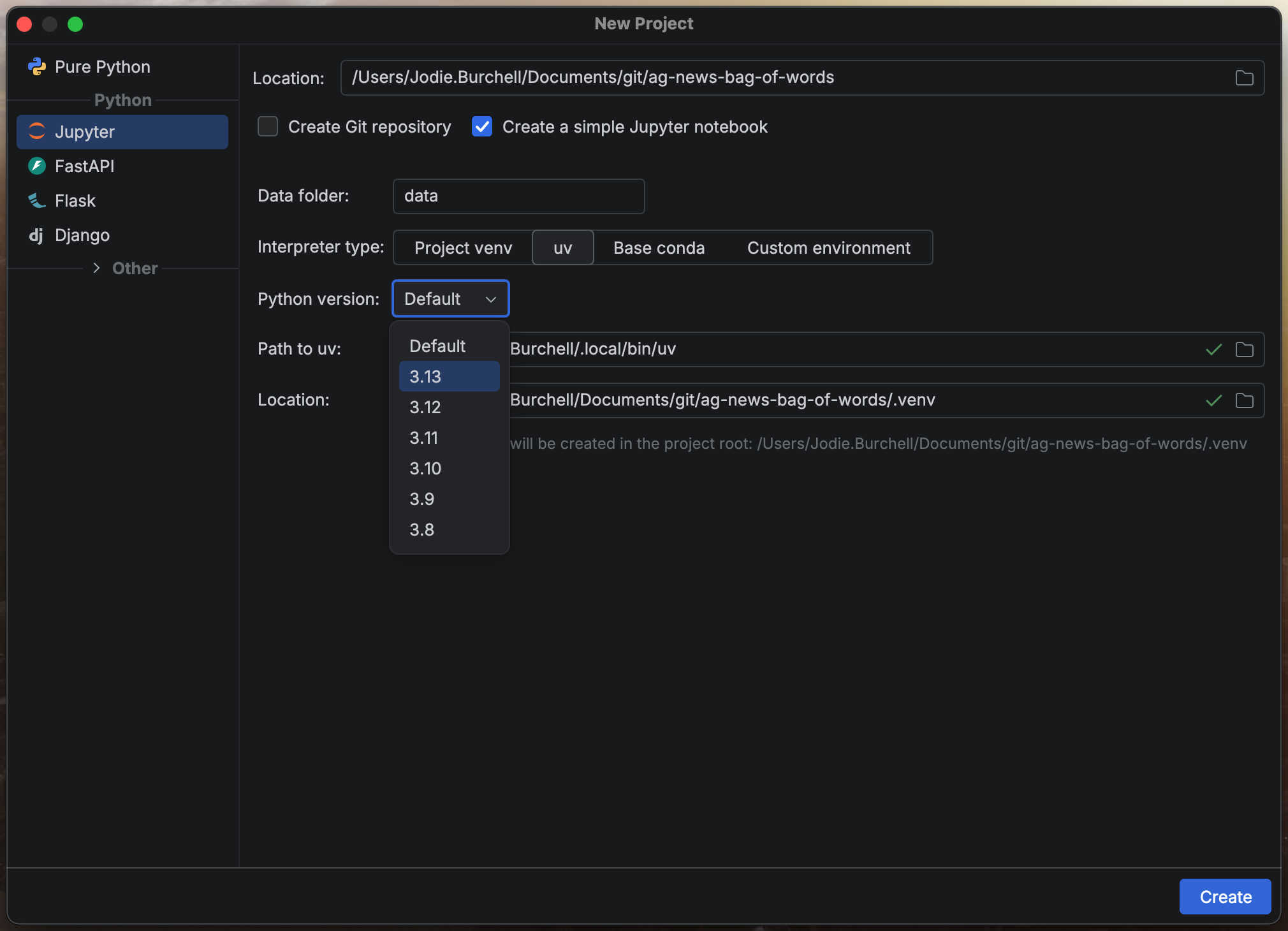
To get started in PyCharm, open the Projects and Files tool window and select New… > New Project…. Since this is a data science project, we can use PyCharm’s built-in Jupyter project type, which sets up a sensible default structure for us.
During project configuration, you’ll be asked to choose a Python interpreter. By default, PyCharm uses uv and lets you select from a range of Python versions, though all major dependency management systems are supported: pip, Anaconda, Pipenv, Poetry, and Hatch. Every project is automatically created with an attached virtual environment, so your setup will be ready to go each time you reopen the project.
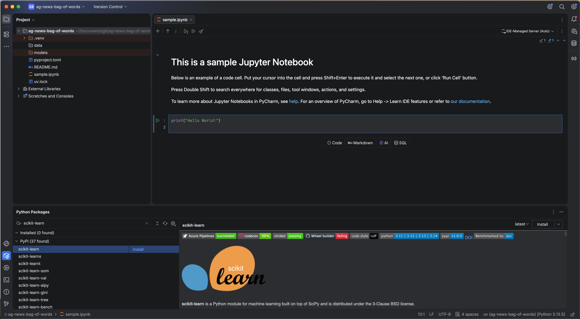
With the project configured, we can install our dependencies via the Python Packages tool window. Simply search for a package by name, select it from the list, and install your desired version directly into the virtual environment. You can also see the same information about the package you’d find on PyPI directly within the IDE. For this project, we’ll need pandas and Numpy, along with datasets from Hugging Face, scikit-learn, Pytorch, and spaCy.
Implementing bag-of-words with PyCharm
There are many versions of this dataset online. We’ll be using one of the versions hosted on Hugging Face Hub.
Loading and preparing the data
We’ll use Hugging Face’s datasets package to download this dataset.
from datasets import load_dataset
ag_news_all = load_dataset("sh0416/ag_news")
This gives us a Hugging Face DatasetDict object. If we look at it, we can see it contains a training dataset with 120,000 news articles, and a test dataset containing 7,600 articles.
As we’ll be training a model, we also need a validation set. We’ll convert the training and test sets to pandas DataFrames, and use the train_test_split method from scikit-learn to create the validation set from the training data.
We now have a validation set with 12,000 articles, and a training set with 108,000 articles.
Training set: 108000 samples
Validation set: 12000 samples
For those of you new to machine learning, you might be wondering why we need all of these different datasets. The reason for this is to make sure we have a good idea that our model will generalize well and perform as expected on unseen data. The training set is the only data the model ever learns from directly. The validation set is used to monitor how the model is performing on unseen data as we make modeling decisions, such as choosing how many epochs to train for, how large to make the hidden layer, or which preprocessing steps to apply (we’ll see all of this later). This means that we look at validation performance repeatedly while building the model, and this increases the risk that our choices gradually become tuned to the quirks of that particular split. This is why we need a third set (the test set), which we keep completely locked away until we’ve finished all modeling decisions and want a single, unbiased estimate of how well our model will perform on new data. Using the test set for anything other than this final evaluation would give us an overly optimistic picture of our model’s real-world performance.
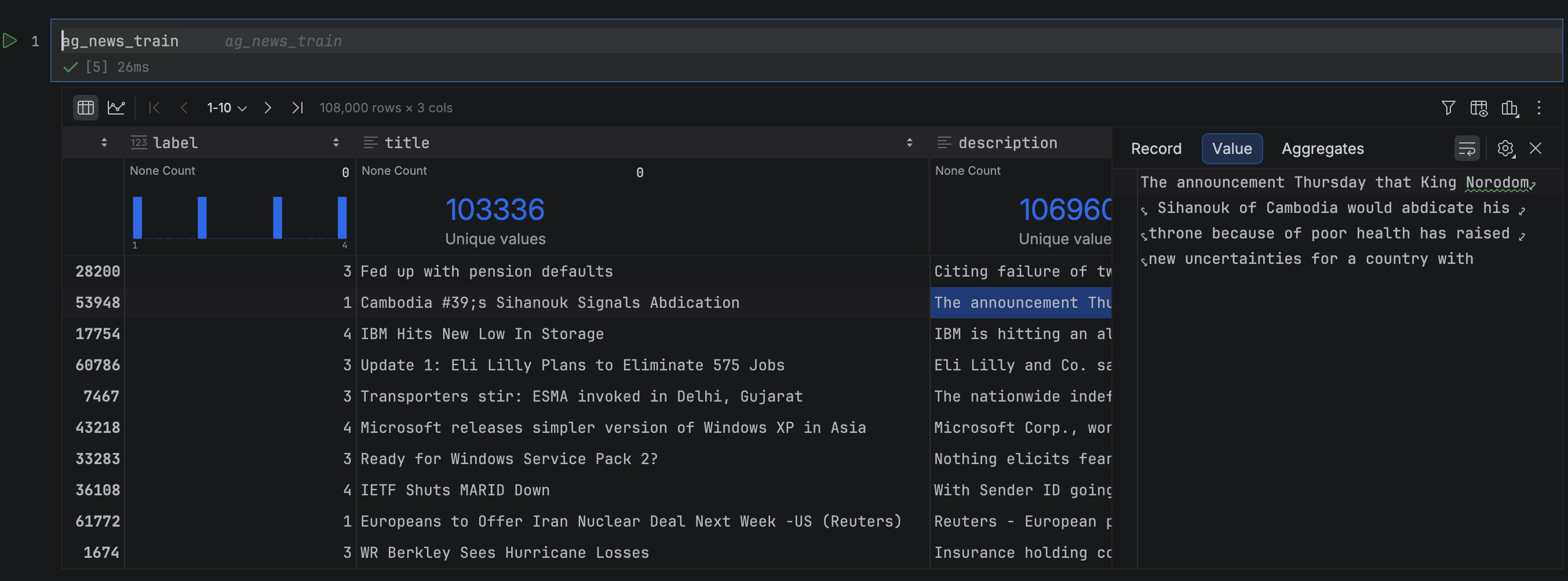
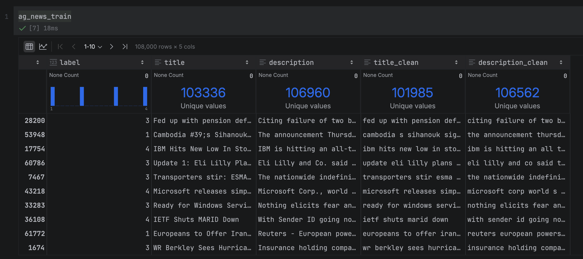
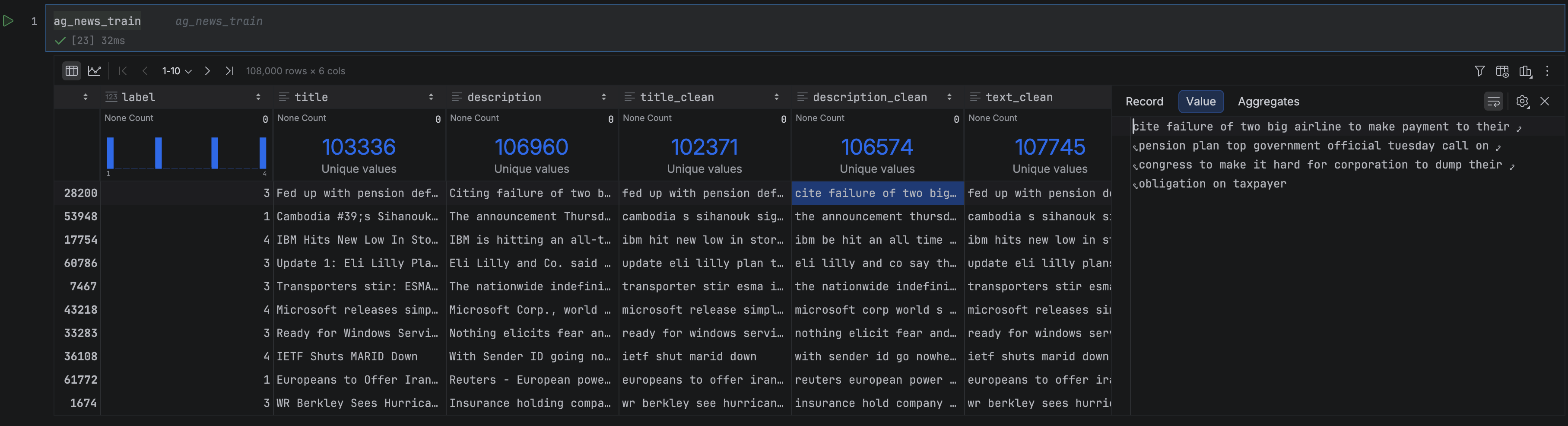
Let’s now inspect our datasets. PyCharm Pro has a lot of built-in features that make working with DataFrames easier, a few of which we’ll see soon. In this DataFrame, we have three columns: The article title and description, the article text, and the label indicating which of the four news categories the article belongs to. You can open any of the DataFrame cells in the Value Editor to see its full text, or widen the column to prevent truncation, both of which are useful for a quick visual inspection.
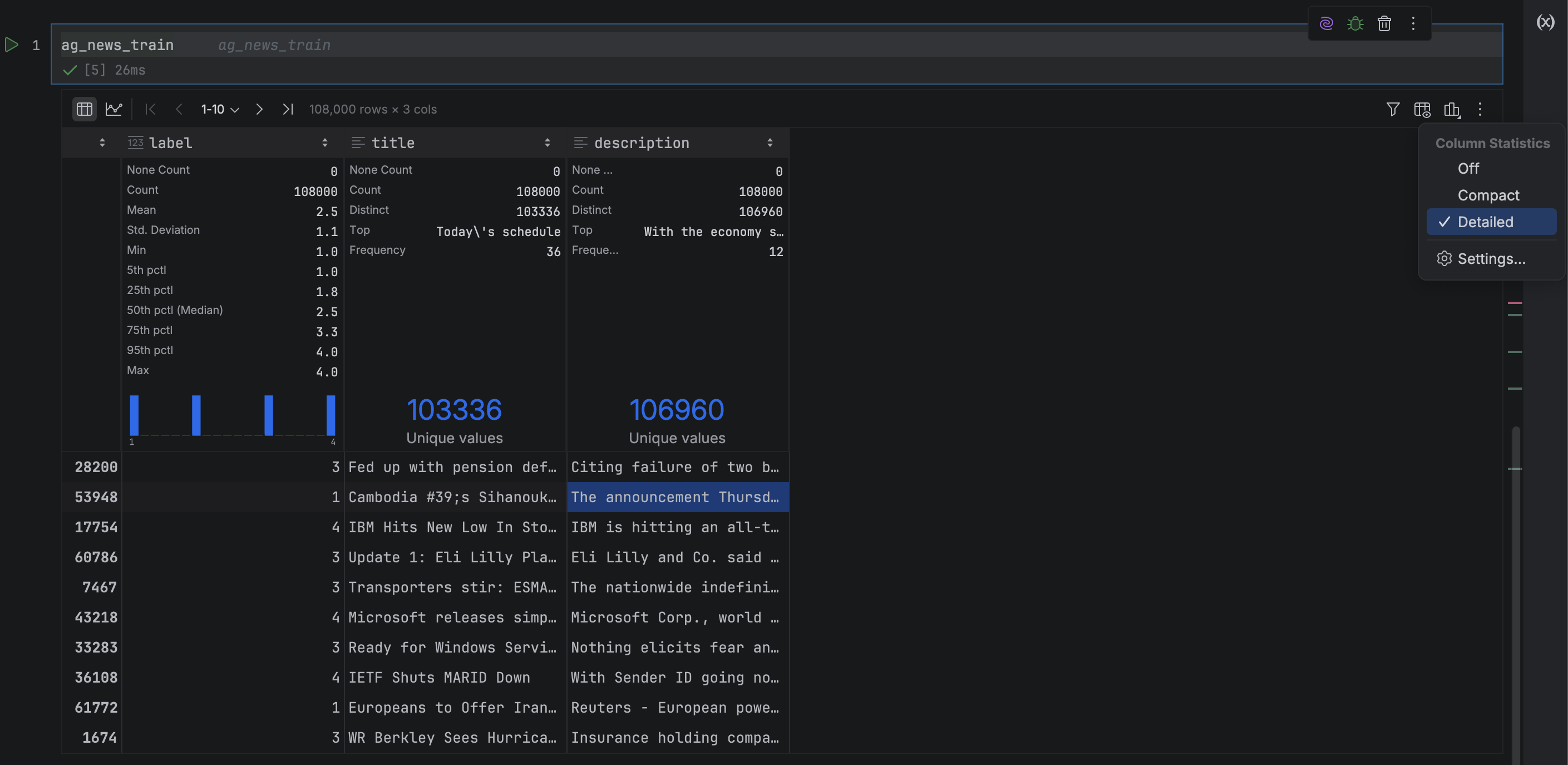
At the top of each column, PyCharm displays column statistics, giving you an at-a-glance summary of the data. Switching from Compact to Detailed mode via Show Column Statistics gives you rich summary statistics about each column, and saves you from writing a lot of pandas boilerplate to get it! From these statistics, we can see that our training set is evenly split across the news categories (which is very handy when training a model). We can also see that some headlines and descriptions are not unique, which may introduce noise when classifying these duplicates.
The first step in preparing the data is basic string cleaning, which normalizes the text and reduces meaningless token variation. For instance, without cleaning, “Natural” and “natural” would be treated as two separate vocabulary entries, as we noted earlier.
We’ll apply four cleaning steps: lowercasing, punctuation removal, number removal, and whitespace normalization. There are different string cleaning steps you can apply depending on the language and use case, but for English-language texts, these tend to be very standard. Let’s go ahead and write a function to do this.
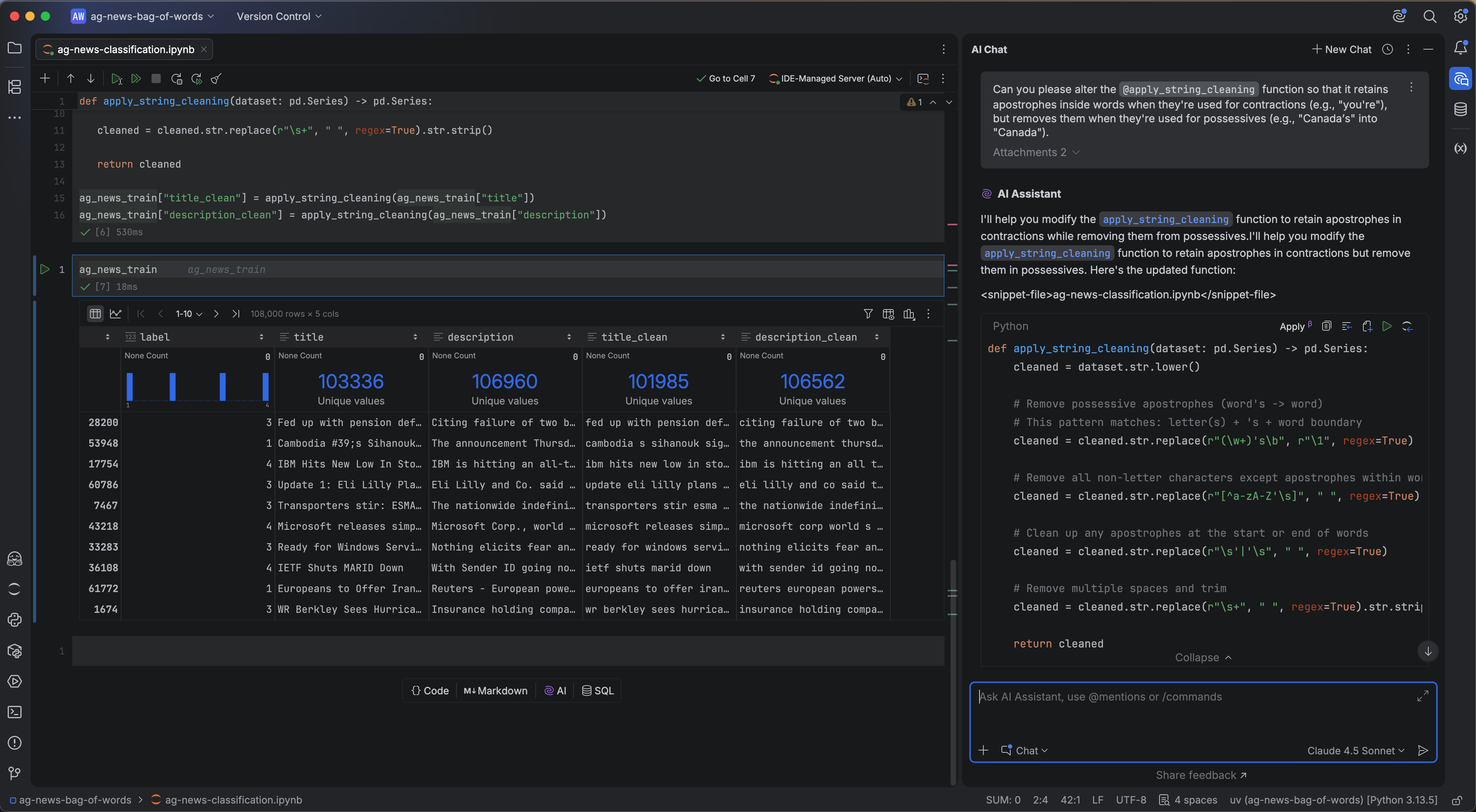
This mostly works, but there’s one issue: The regex strips apostrophes entirely, turning contractions like “you’re” into “you re” and possessives like “Canada’s” into “Canada s”. The cleanest fix is a regex that preserves apostrophes in contractions while removing possessive endings, but this is not the most enjoyable thing to write by hand.
This is where PyCharm’s built-in AI Assistant comes in. Open the chat window via the AI Chat icon on the right-hand side of the IDE and enter the following prompt:
Can you please alter the @apply_string_cleaning function so that it retains apostrophes inside words when they’re used for contractions (e.g., “you’re”), but removes them when they’re used for possessives (e.g., “Canada’s” into “Canada”).
The @ notation lets you reference specific files or objects in your IDE without copying and pasting code into the prompt, including Jupyter variables like datasets and functions.
I ran this against Claude Sonnet 4.5, though JetBrains AI supports a wide range of models from OpenAI, Anthropic, Google, and xAI, as well as open models via Ollama, LM Studio, and OpenAI-compatible APIs. Below is the updated function it returned:
def apply_string_cleaning(dataset: pd.Series) -> pd.Series:
    cleaned = dataset.str.lower()

    # Remove possessive apostrophes (word's -> word)
    # This pattern matches: letter(s) + 's + word boundary
    cleaned = cleaned.str.replace(r"(w+)'sb", r"1", regex=True)

    # Remove all non-letter characters except apostrophes within words
    cleaned = cleaned.str.replace(r"[^a-zA-Z's]", " ", regex=True)

    # Clean up any apostrophes at the start or end of words
    cleaned = cleaned.str.replace(r"s'|'s", " ", regex=True)

    # Remove multiple spaces and trim
    cleaned = cleaned.str.replace(r"s+", " ", regex=True).str.strip()

    return cleaned

ag_news_train["title_clean"] = apply_string_cleaning(ag_news_train["title"])
ag_news_train["description_clean"] = apply_string_cleaning(ag_news_train["description"])
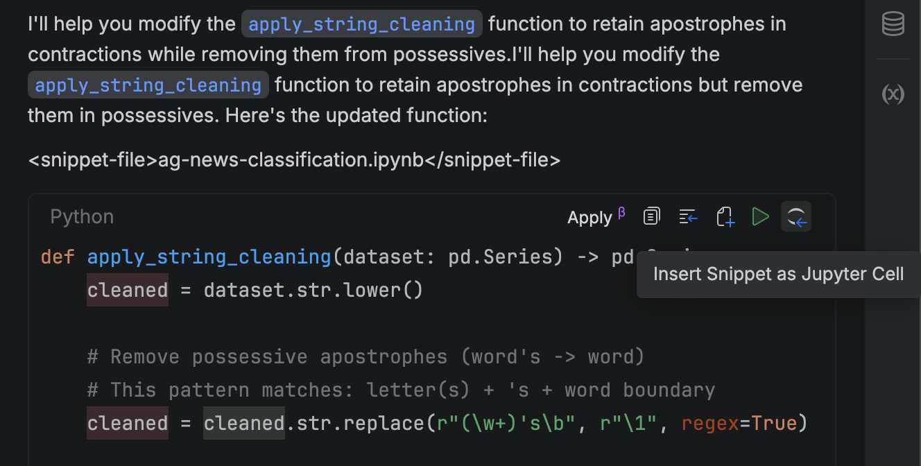
We can insert this into our Jupyter notebook directly by clicking on Insert Snippet as Jupyter Cell in the AI chat.
Once we run this updated function on our raw text, we get the correct result:
text
text_clean
Don’t stand for racism – football chief
don’t stand for racism football chief
Canada’s Barrick Gold acquires nine per cent stake in Celtic Resources (Canadian Press)
canada barrick gold acquires nine per cent stake in celtic resources canadian press
We can see the contraction “don’t” is correctly preserved in the first example, but the possessive “Canada’s” has been removed. We apply this to both the training and validation datasets using the same function, so that the cleaning is consistent across both splits:
The process has two distinct steps. First, .fit() scans the training data and builds a vocabulary by identifying every unique word and assigning it a fixed index position (for example, “government” = column 8,901). The result is a mapping of 59,544 unique words, which you can think of as the column headers for our eventual matrix.
Second, .transform() uses that vocabulary to convert each headline into a numerical vector, counting how many times each vocabulary word appears and placing that count at the corresponding index position.
The reason these are two separate steps is important: When we later process our validation and test data, we’ll call .transform() using the vocabulary learned from the training set. This ensures that all three splits share a consistent feature space. If we re-ran .fit() on the test data, we’d get a different vocabulary, and the model’s predictions would be meaningless.
With the vectorizer fitted and our training data transformed, we can start exploring what we’ve actually built. Let’s first take a look at the vocabulary. CountVectorizer stores it as a dictionary mapping each word to its index position, accessible via vocabulary_:
This confirms that our vocabulary contains 59,544 unique words. Browsing through it, you can start to guess what kinds of terms appear frequently in the different types of news. Country names feature heavily in the “world” news category, terms like “football” and “cricket” in the “sports” news category, terms like “profit” and “losses” in the “business” news category, and company names like “Google” and “Microsoft” in the “science/technology” category.
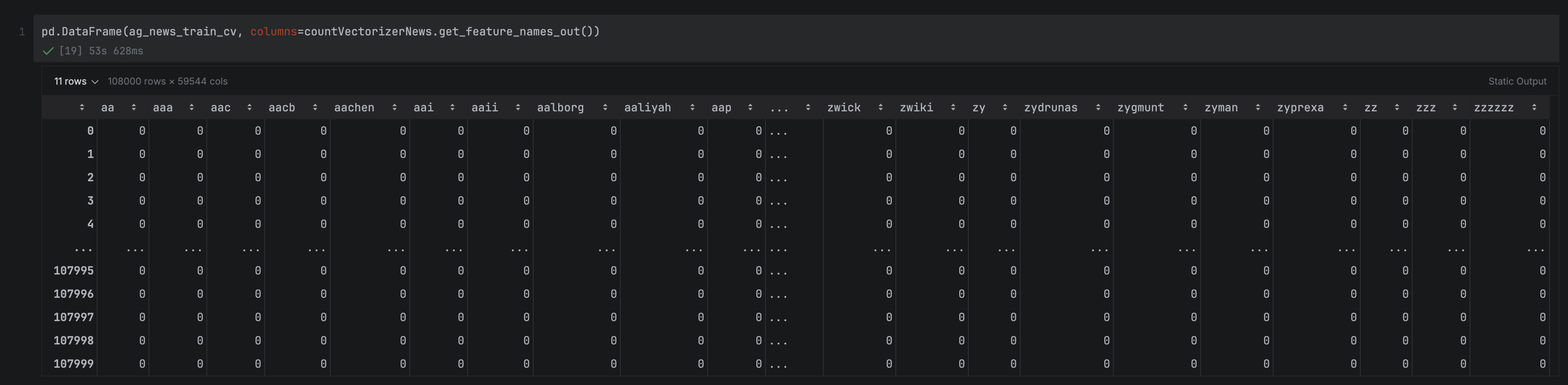
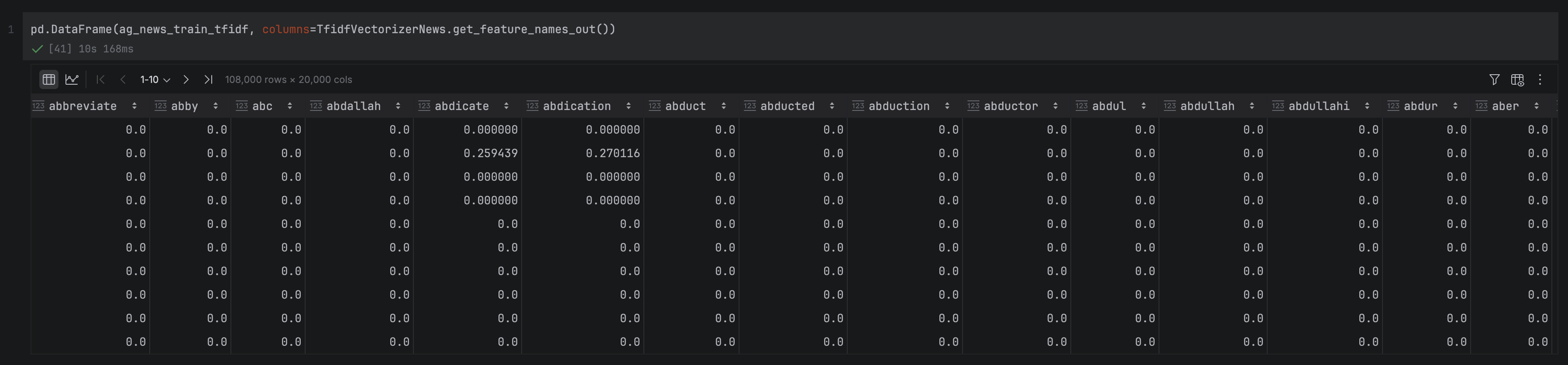
Next, let’s inspect the feature matrix itself. ag_news_train_cv is a NumPy array with one row per headline and one column per vocabulary word, giving us a matrix of shape (108,000 × 59,544). We can wrap it in a DataFrame to make it easier to inspect in PyCharm’s DataFrame viewer:
As expected, the matrix is very sparse. Most values are zero, since any individual headline only contains a small fraction of the full vocabulary. In fact, you might have noticed that the number of columns is two-thirds of the number of rows, which is never good for a feature matrix. We’ll explore how to reduce the dimensionality of the feature space in a later section.
Note that we also need to apply this vectorization to the validation dataset before moving on to modeling. Importantly, we are only applying the .transform method to the validation set, as we already trained it on the training dataset.
Before we move onto reducing down the dimensionality of our feature space, let’s explore the distribution of the words in our corpus. This can help us to understand the most common and rare words, and how we might use this to further process our data to amplify the signal-to-noise ratio.
Word frequency plots
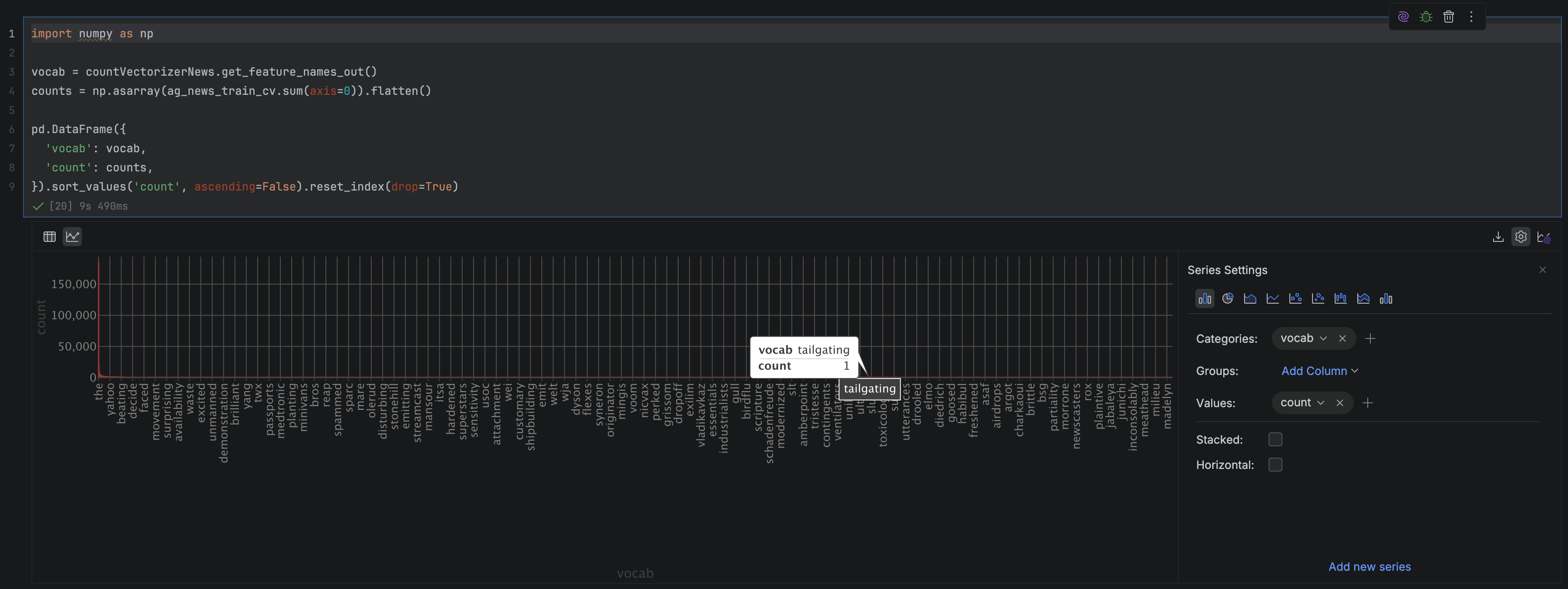
We’ll start by creating a DataFrame that aggregates word counts across all headlines and ranks them by frequency:
First, we retrieve the vocabulary in index order using get_feature_names_out(), so each word lines up with its corresponding column in the feature matrix. We then sum the matrix column-wise (that is, across all documents) to get the total number of times each word appears in the training set. Finally, we wrap these two arrays into a DataFrame and sort by count, giving us a ranked list of the most frequent terms.
Once this DataFrame is displayed in PyCharm, we can easily turn it into a visualization without writing a single line of code. By clicking on the Chart View button in the top left-hand corner of the DataFrame, we can explore a range of ways of visualizing our data. Go to Show Series Settings in the top right-hand corner, and adjust the parameters to get the count frequencies of the words: we set the X axis value to “vocab” (and change group and sort to none), the Y axis value to “count”, and the chart type to “Bar”.
Hovering over this chart, we can see that it has a very long-tailed distribution, which is very typical of vocabulary frequencies (this is actually so typical that it is described in something called Zipf’s law). This means that the majority of our words very rarely occur in the text, and in fact, if we hover over the right-hand side of the chart, it looks like around a third of our vocabulary terms are only used once!
On the other hand, when we hover over the left-hand side of the chart, we can see that this is dominated by very common words, prepositions, and articles, such as “to”, “in”, “the”, and “you”. These words don’t really carry any meaning and pretty much occur in every text, so they’re unlikely to be useful for our classification task.
Let’s have a look at some things we can do to clean up our feature space and help our semantically meaningful words stand out a bit more.
Advanced bag-of-words techniques
The basic BoW pipeline we’ve built so far is a solid foundation, but there are several techniques that can meaningfully improve its quality. This section walks through the most important ones. We’ll only be using a selection of them in our project, but you can investigate which of these seem appropriate when building your own project.
Stop word removal
Stop words are extremely common words that appear frequently across all kinds of text but carry little meaningful information. This includes words like “the”, “is”, “and”, “of”, as we saw in the histogram in the previous section. They inflate vocabulary size without adding signal, so removing them is one of the most straightforward ways to improve your BoW representation. NLTK provides a built-in stop word list for English and many other languages.
Stemming and lemmatization
Another issue you might have noticed in our vocabulary is that words that are semantically equivalent have different syntactic forms, meaning that while they should be treated as the same token, they occupy additional token slots. We can resolve this through two techniques: stemming and lemmatization. Stemming reduces words to their root form using simple rule-based truncation (e.g. “running” → “run”), while lemmatization takes a linguistic approach, mapping words to their dictionary base form. Lemmatization is slower but generally produces cleaner results, particularly for irregular word forms.
TF-IDF
Term frequency-inverse document frequency (TF-IDF) is an extension of basic count vectorization that weights each word by how informative it actually is. A word that appears frequently in one document but rarely across the corpus receives a high weight; a word that appears everywhere receives a low one. This neatly addresses one of the core weaknesses of raw count vectors: common but uninformative words can dominate the feature space even after stop-word removal.
N-grams
Standard BoW treats each word independently, which means it misses phrases whose meaning depends on word combinations. A classic example of this is “machine learning”, which has a distinct meaning to “machine” + “learning”. N-grams address this by treating sequences of adjacent words as single tokens, so a bigram model would capture “machine learning” as a feature in its own right. The trade-off is a much larger vocabulary, so in practice, bigrams are most commonly used, with trigrams reserved for cases where capturing longer phrases is important.
Handling out-of-vocabulary words
When you apply your fitted vectorizer to new data, any words not present in the training vocabulary are silently ignored by default. For many tasks, this is acceptable, but if your production data is likely to continue introducing new terms that carry meaningful signal, it’s worth considering alternatives. One common approach is to reserve a special <UNK> token to represent unseen words, which at least preserves the information that something unfamiliar appeared, even if its identity is unknown and multiple (perhaps unrelated) words are collapsed onto the same token.
However, LLMs, with their more flexible approach to tokenization, tend to be a better choice if out-of-vocabulary words will be a major issue for your model once it is in production.
Dimensionality reduction
Even after stop word removal and other cleaning steps, BoW feature matrices are typically very high-dimensional and sparse. Two widely used techniques can help. Reducing to the top-N most frequent terms is the simplest approach, discarding low-frequency words that are unlikely to generalize well. For a more principled reduction, techniques like principal component analysis (PCA) or latent semantic analysis (LSA) project the feature matrix into a lower-dimensional space, compressing the representation while preserving as much of the meaningful variance as possible.
Feature selection techniques
Rather than reducing dimensionality arbitrarily, feature selection methods identify and retain only the features most relevant to your specific task. Chi-squared testing measures the statistical dependence between each term and the target label, making it well-suited to classification tasks. Mutual information takes a similar approach, scoring each feature by how much it reduces uncertainty about the class. Both methods can substantially reduce vocabulary size while preserving model performance.
Applying bag-of-words to a real-world problem
Let’s now continue the example we started earlier. We’re going to take the work we’ve done on our AG News text classification task and take it to its completion by building a model.
A common way to build a model using encoded text is neural networks, where each of the words in the vocabulary is treated as a feature, and the categories we want to predict (in our case, the news category) are the output. We’ll start by building a baseline model that applies only string cleaning and encoding to the text.
I had originally written this model in Keras, as part of a previous BoW project from a couple of years ago. However, that code was now out of date. In order to update it and adapt it to Pytorch, I asked JetBrains AI to do the following:
Please update this neural network from Keras to Pytorch, making improvements to make the code as reusable as possible.
This gave us the following successful port of the code:
import torch
import torch.nn as nn
import torch.optim as optim
from torch.utils.data import TensorDataset, DataLoader

class MulticlassClassificationModel(nn.Module):
   def __init__(self, input_size: int, hidden_layer_size: int, num_classes: int = 4):
       super(MulticlassClassificationModel, self).__init__()
       self.fc1 = nn.Linear(input_size, hidden_layer_size)
       self.relu = nn.ReLU()
       self.fc2 = nn.Linear(hidden_layer_size, num_classes)

   def forward(self, x):
       x = self.fc1(x)
       x = self.relu(x)
       x = self.fc2(x)
       return x

def train_text_classification_model(
       train_features: np.ndarray,
       train_labels: np.ndarray,
       validation_features: np.ndarray,
       validation_labels: np.ndarray,
       input_size: int,
       num_epochs: int,
       hidden_layer_size: int,
       num_classes: int = 4,
       batch_size: int = 1920,
       learning_rate: float = 0.001) -> MulticlassClassificationModel:

   # Convert labels to 0-indexed (AG News has labels 1,2,3,4 -> need 0,1,2,3)
   train_labels_indexed = train_labels - 1
   validation_labels_indexed = validation_labels - 1

   # Convert numpy arrays to PyTorch tensors
   X_train = torch.FloatTensor(train_features.copy())
   y_train = torch.LongTensor(train_labels_indexed.copy())
   X_val = torch.FloatTensor(validation_features.copy())
   y_val = torch.LongTensor(validation_labels_indexed.copy())

   # Create datasets and dataloaders
   train_dataset = TensorDataset(X_train, y_train)
   train_loader = DataLoader(train_dataset, batch_size=batch_size, shuffle=True)

   # Initialize model, loss function, and optimizer
   model = MulticlassClassificationModel(input_size, hidden_layer_size, num_classes)
   criterion = nn.CrossEntropyLoss()
   optimizer = optim.RMSprop(model.parameters(), lr=learning_rate)

   # Training loop
   for epoch in range(num_epochs):
       model.train()
       train_loss = 0.0
       correct_train = 0
       total_train = 0

       for batch_features, batch_labels in train_loader:
           # Forward pass
           outputs = model(batch_features)
           loss = criterion(outputs, batch_labels)

           # Backward pass and optimization
           optimizer.zero_grad()
           loss.backward()
           optimizer.step()

           # Calculate training metrics
           train_loss += loss.item()
           _, predicted = torch.max(outputs, 1)
           correct_train += (predicted == batch_labels).sum().item()
           total_train += batch_labels.size(0)

       # Validation
       model.eval()
       with torch.no_grad():
           val_outputs = model(X_val)
           val_loss = criterion(val_outputs, y_val)
           _, val_predicted = torch.max(val_outputs, 1)
           correct_val = (val_predicted == y_val).sum().item()
           total_val = y_val.size(0)

       # Print epoch metrics
       train_acc = correct_train / total_train
       val_acc = correct_val / total_val
       print(f'Epoch [{epoch+1}/{num_epochs}], '
             f'Train Loss: {train_loss/len(train_loader):.4f}, '
             f'Train Acc: {train_acc:.4f}, '
             f'Val Loss: {val_loss:.4f}, '
             f'Val Acc: {val_acc:.4f}')

   return model

def generate_predictions(model: MulticlassClassificationModel,
                       validation_features: np.ndarray,
                       validation_labels: np.ndarray) -> list:
   model.eval()

   # Convert to tensors
   X_val = torch.FloatTensor(validation_features.copy())

   with torch.no_grad():
       outputs = model(X_val)
       _, predicted = torch.max(outputs, 1)

   # Convert back to 1-indexed labels to match original dataset
   predicted_labels = (predicted.numpy() + 1)

   print("Confusion Matrix:")
   print(pd.crosstab(validation_labels, predicted_labels,
                     rownames=['Actual'], colnames=['Predicted']))
   return predicted_labels.tolist()
Let’s walk through this code step-by-step to understand how we’re going to train our text classifier.
The model architecture
MulticlassClassificationModel is a simple two-layer feedforward neural network. It takes a BoW vector as input, with each feature being a vocabulary word, and passes it through two sequential transformations to produce a prediction. The first layer (fc1) compresses this high-dimensional input down to a smaller intermediate representation, whose size we control via hidden_layer_size. A ReLU activation is then applied, which introduces a small amount of mathematical complexity that allows the model to learn patterns that a simple weighted sum couldn’t capture. The second layer (fc2) takes this intermediate representation and maps it down to four output values, one per news category, where the category with the highest value becomes the model’s prediction.
Training and validation
train_text_classification_model handles the full training loop. It starts with a small amount of housekeeping: The AG News labels run from 1 to 4, but PyTorch expects 0-indexed classes, so these are shifted down by 1. The features and labels are then converted to PyTorch tensors, and a DataLoader is created to feed the training data to the model in batches.
Each epoch, the model processes the training data batch by batch. For each batch, it runs a forward pass to generate predictions, computes the cross-entropy loss against the true labels, and then runs a backward pass to update the model weights via the RMSprop optimizer. At the end of every epoch, the model switches into evaluation mode and runs inference over the full validation set, printing the training and validation loss and accuracy so we can monitor how training is progressing.
Generating predictions
Once training is complete, generate_predictions runs the trained model on a held-out dataset and returns the predicted class for each article. It also prints a confusion matrix, which gives us a breakdown of which categories the model is getting right and where it’s getting confused, which is a much more informative picture than accuracy alone.
Running the baseline
We can now train the baseline model. We pass in the raw count-vectorized training and validation features, specify an input size equal to the vocabulary size (59,544 columns), train for two epochs, and use a hidden layer of 5,000 nodes.
Even with the very basic data preparation we did, we can see we’ve performed very well on this prediction task, with around 92% accuracy. The confusion matrix shows that the model seems to have the easiest time distinguishing between category two (sports) and the other topics, and the hardest time distinguishing between category three (business) and category four (science/technology). This makes sense, as the words used to describe sports are very distinct and unlikely to be used in other contexts (things like football), whereas there is likely to be overlapping vocabulary between business and technology (especially company names).
As we saw above, there is a lot we can do to improve the signal-to-noise ratio in BoW modeling. Let’s apply four commonly used techniques to our data and see whether this improves our predictions: lemmatization, stop word removal, limiting our vocabulary to the top N terms, and TF-IDF weighting. As you’ll see, all of these can be done relatively simply using inbuilt functions in packages such as spaCy and scikit-learn.
Lemmatization
As we discussed earlier, lemmatization collapses inflected word forms into a single vocabulary entry by mapping each word to its dictionary base form, which both shrinks the vocabulary and concentrates the signal for each concept into a single feature. We’ll use spaCy for this, which first requires downloading its small English language model:
Our lemmatise_text function passes each text through spaCy’s NLP pipeline using nlp.pipe(), which processes them in batches of 1,000 for efficiency. For each document, it extracts the .lemma_ attribute of every token and joins them back into a single string. One small detail worth noting: we preserve the original DataFrame index when constructing the output Series, so that rows stay correctly aligned when we assign the results back.
We apply lemmatization before string cleaning, since spaCy needs the original casing and punctuation to correctly identify grammatical structure. For example, “running” and “Running” lemmatize to the same thing, but removing punctuation first can confuse the parser. Once lemmatized, we pass the output through apply_string_cleaning as before:
We apply this separately to the title and description columns before concatenating them into a single text_clean field. As you can see, we do this for both the training and validation sets using the same function, so that lemmatization is applied consistently across both splits.
Removing stop words
As with lemmatization, we covered the motivation for stop word removal earlier: Words like “the”, “is”, and “of” appear so frequently across all texts that they add noise rather than signal to our feature matrix. Here we’ll actually apply it to our data.
def remove_stopwords(texts: pd.Series) -> pd.Series:
   texts = texts.fillna("").astype(str)

   filtered_texts = []
   for doc in nlp.pipe(texts, batch_size=1000):
       filtered_texts.append(
           " ".join(token.text for token in doc if not token.is_stop)
       )

   return pd.Series(filtered_texts, index=texts.index)
Our remove_stopwords function again uses nlp.pipe() to process texts in batches. For each document, it filters out any token where spaCy’s is_stop attribute is True, and joins the remaining tokens back into a string. Conveniently, spaCy handles stop word detection using the same pipeline we already loaded for lemmatization, so no additional setup is needed.
We apply this to the already-cleaned and lemmatized text_clean column for both the training and validation sets, so the stop word removal builds directly on our previous preprocessing steps and is applied consistently across both splits.
The final two improvements we’ll apply are limiting the vocabulary size and switching from raw count vectorization to TF-IDF weighting. Conveniently, scikit-learn’s TfidfVectorizer handles both in a single step.
Recall from earlier that TF-IDF downweights words that appear frequently across many documents while upweighting words that are distinctive to particular documents. This cleans up uninformative words that don’t quite qualify as stopwords, but add little useful information to our dataset. The max_features=20000 argument caps the vocabulary at the 20,000 most frequent terms after TF-IDF scoring, which discards the long tail of rare words that are unlikely to generalize well and brings our feature matrix down to a much more manageable size. (The choice of 20,000 words is arbitrary. We could have easily used a smaller or larger number, depending on our dataset and use case.)
As with CountVectorizer, we fit only on the training data and then use that fixed vocabulary to transform both the training and validation sets:
Compared to our baseline feature matrix of 59,544 columns filled almost entirely with zeros, this is considerably leaner. We now have 20,000 columns of weighted scores that better reflect each word’s actual importance to the document it appears in. It is still relatively sparse, but we can see from both the feature matrix and the vocabulary list that it is much more focused on semantically rich words.
Fitting the revised model
With our improved features in hand, we can now retrain the model. The call is identical to before, except we pass in the TF-IDF feature matrices instead of the raw count vectors, and the input size is now 20,000 rather than 59,544:
Epoch [1/2], Train Loss: 0.3183, Train Acc: 0.8932, Val Loss: 0.2301, Val Acc: 0.9225
Epoch [2/2], Train Loss: 0.1512, Train Acc: 0.9475, Val Loss: 0.2332, Val Acc: 0.9243
Confusion Matrix - Raw Counts:
Predicted     1     2     3     4
Actual
1          2703    71   121   105
2            20  2955    13    12
3            68    19  2691   222
4            77    17   163  2743
The results are actually very encouraging! Our overall validation accuracy is essentially unchanged at around 92%, but we’ve achieved this with a feature matrix that is less than a third of the size. This suggests that the extra vocabulary in the baseline (including the stop words) was contributing to noise rather than signal. Reducing the size of the feature matrix makes our model more stable, less prone to overfitting, and much more manageable to deploy.
Looking at the confusion matrix, the pattern of errors is similar to before: Sports (category two) is the easiest category to classify, with 98.5% accuracy, while Business (category three) and Science/Technology (category four) remain the hardest to separate, with around 7% of articles in each category being misclassified as the other. This is consistent with what we saw in the baseline, so it seems that the preprocessing improvements have tightened things up at the margins, but the fundamental difficulty of the Business/Technology boundary is a property of the data rather than the feature representation.
Applying our model to the test set
Finally, we need to validate that our model performs as well on the test set as it does on the validation set. Up to this point, we’ve deliberately kept the test set locked away. As mentioned earlier, if we had been making modeling decisions based on test set performance, we’d risk inadvertently overfitting our choices to it, and our final accuracy estimate would be optimistic.
The preprocessing steps must be applied in exactly the same order as for the training and validation data: lemmatization, string cleaning, concatenation of title and description, and stop-word removal. Crucially, we also call .transform() rather than .fit_transform() on the test text, using the vocabulary learned from the training data:
The test accuracy of 91.8% is very close to the 92.4% we saw on the validation set, which is a reassuring sign that our model has generalized well rather than overfitting to the validation data. The confusion matrix tells the same story as before: Sports (category two) remains the easiest category to classify, with only 30 misclassified articles out of 1,900, while the Business/Technology boundary continues to be the main source of errors, with around 8% of articles in each category being misclassified as the other. The consistency between validation and test results gives us confidence that these error patterns reflect genuine properties of the data rather than artifacts of any particular split.
Limitations and alternatives
Loses word order information
The most fundamental limitation of the bag-of-words model is right there in the name: it treats text as an unordered collection of words, discarding all sequence information. This means “the dog bit the man” and “the man bit the dog” produce identical vectors, even though they describe very different events. For many classification tasks, this doesn’t matter much, but for tasks that require understanding the relationship between words, such as question answering or natural language inference, the loss of word order is a serious handicap.
Ignores semantics and context
BoW has no notion of word meaning or context. Each word is simply a column in a matrix, entirely independent of every other word. This creates two related problems. First, synonyms are treated as completely distinct features: “cheap” and “inexpensive” contribute nothing to each other’s signal, even though they mean the same thing. Second, words with multiple meanings are treated as a single feature regardless of context: “bank” means the same thing whether it appears in a sentence about rivers or finance. Both of these issues limit how well BoW representations can capture the actual semantics of a text.
Can result in large, sparse vectors
As we saw in our own example, even a moderately sized corpus of news headlines can produce a vocabulary of nearly 60,000 unique terms. The resulting feature matrix has one column per vocabulary word, but any individual document only uses a tiny fraction of them, leaving the vast majority of values at zero. This sparsity creates two practical problems: The matrices can consume a large amount of memory if stored densely, and the high dimensionality can make it harder for models to find meaningful patterns, a phenomenon sometimes called the curse of dimensionality.
Alternatives
If BoW’s limitations are a bottleneck for your task, there are several well-established alternatives worth considering.
Word embeddings (Word2Vec and GloVe) address the semantics problem by representing each word as a dense vector in a continuous space, where similar words are geometrically close to each other. They capture distributional meaning far more richly than BoW, and are a natural next step when synonym handling or word similarity matters. Doc2Vec extends this idea to produce embeddings for entire documents rather than individual words.
Transformer-based models (BERT and GPT) go further still, generating contextual representations where the same word receives a different vector depending on the surrounding text. This handles polysemy directly and captures complex long-range dependencies between words. The trade-off is substantially higher computational cost and complexity compared to BoW.
Topic models like latent Dirichlet allocation (LDA) take a different angle entirely. Rather than encoding documents for downstream classification, they are generative models that discover latent thematic structure in a corpus. This is useful when your goal is exploration and interpretation rather than prediction.
For tasks where BoW already performs well, as we saw here with AG News, the added complexity of these approaches may not be worth the cost. BoW remains a strong baseline, and it’s always worth establishing how far it can take you before reaching for heavier machinery.
Get started with PyCharm today
In this post, we’ve covered a lot of ground: from the fundamentals of the bag-of-words model and how it converts text into numerical vectors, through to building and iteratively improving a real text classification pipeline on the AG News dataset. Along the way, we’ve seen how preprocessing steps like lemmatization, stop word removal, vocabulary capping, and TF-IDF weighting can meaningfully improve the efficiency of your feature representation, and how PyCharm’s DataFrame viewer, column statistics, chart view, and AI Assistant make each of these steps faster and easier to inspect and debug.
If you’d like to try this yourself, PyCharm Pro comes with a 30-day trial. As we saw in this tutorial, its built-in support for Jupyter notebooks, virtual environments, and scientific libraries means you can go from a blank project to a working NLP pipeline with minimal setup friction, leaving you free to focus on the fun parts.
You can find the full code for this project on GitHub. If you’re interested in exploring more NLP topics, check out our recent blogs here.
Another four hours down in the Minecraft world with Kiwi-chan, and it’s been a steady, if slightly repetitive, climb! We’re still firmly focused on the core survival loop: get wood, build a base. However, Kiwi-chan is very insistent on finding oak logs, even when they aren’t around. The “OAK OBSESSION BAN” rule is getting a workout, forcing the AI to switch to birch logs when oak proves elusive.
The logs show a fascinating pattern of repeated failures with gather_oak_log, followed by a switch to gather_birch_log. It’s a good sign that the system is responding to the environment and attempting to adapt. We’ve also hit a “BOREDOM TRIGGERED” alert – apparently, repeatedly digging dirt gets old, even for an AI! The Coach (that’s our rule-based decision-making system) is stepping in to diversify tasks.
Debugging continues to be a major focus. We’re seeing a lot of “Code extraction failed” errors, and the AI is struggling with basic tasks like digging dirt. I’ve been manually fixing the generated code, but it’s a constant battle. It’s clear the LLM is still prone to generating syntactically incorrect JavaScript.
The audit rules are proving invaluable. The beforeCount and afterCount checks are catching failed item pickups, and the pathfinding rules are helping to avoid getting stuck. I’ve also reinforced the importance of finding open ground for block placement and avoiding hardcoded coordinates.
Overall, progress is incremental, but the system is learning. The constant cycle of failure, debugging, and adaptation is exactly what we need to build a truly autonomous Minecraft AI. It’s a bit like building Frankenstein’s monster, honestly – lots of patching and hoping it doesn’t turn on me! 😅
Help Kiwi-chan Level Up! 🥝✨
This project is fueled by passion (and a rapidly overheating GPU!). Any contribution, big or small, directly helps me upgrade my melting “Frankenstein” rig to an RTX 3060, which will dramatically improve Kiwi-chan’s processing power and allow for more complex behaviors.
🛡️ Join the inner circle on Patreon (Monthly Support): https://www.patreon.com/15923261/join
☕ Tip me a coffee on Ko-fi (One-time Tip): https://ko-fi.com/kiwitech
This tutorial was written by an external contributor.
Kevin Kimani
Kevin Kimani is a software engineer and technical writer with over three years of experience in software development and documentation. He works across full-stack web development, database design, RESTful API development, and technical writing for engineer audiences. His writing focuses on clear API documentation, tutorials, and how-to guides that help developers understand and use products more easily.
GitHub | X.com
Repository with the companion code for the tutorial
Go to GitHub
As a developer, logging is usually the first technique that you reach for when something goes wrong in your application. You add a few log statements at the start and end of a function and in the exception handlers, and then you get a basic picture of what your application is doing. For simple services that run on a single instance, this approach is usually enough. You can just go through the log file, spot the error, and trace it back to its cause in just a few minutes.
But as your systems grow, that same approach doesn’t work. Logs start to pile up from multiple sources, executions interleave, and the error you’re looking at in the logs doesn’t provide enough information. You can clearly see the error, but you can’t trace it back to what caused it.
In this tutorial, you’ll learn how to move beyond basic logging by instrumenting a Kotlin and Spring Boot backend service with OpenTelemetry. You’ll learn how OpenTelemetry’s tracing model gives you the execution context that logs alone can’t provide. By the end of this guide, you’ll have a working instrumented service and a clear mental model for building more observable backend systems.
Why You Need Next-Level Observability
Modern backend systems are rarely linear. One operation might fan out to several downstream services, retry on failure, or execute concurrently across multiple instances and threads. All these patterns create opportunities for failure that might be hard to explain after the fact. When a background job that processes hundreds of records across overlapping executions errors out, your logs won’t tell you much. You won’t be able to explain which execution the error belonged to or whether the other executions succeeded or failed in the same way.
The lack of execution context creates a gap between seeing the error in your logs and actually understanding what happened leading to it. You just have the error message and a timestamp, but no way to connect it to the broader execution that it belongs to. In a system that runs multiple concurrent job executions, logs from different runs always interleave freely, and thread names get reused by the thread pool. Without a way to uniquely identify each execution, each line of text in your log file is an isolated fact without any reliable way to group it with others that belong to the same run.
Observability gives you a structured view of what your system did and in what order. It does this through traces, which are records of complete operations that contain unique identifiers. You can easily filter your logs by these trace identifiers, and you’ll be able to see the entire history of a specific execution clearly. Metrics add another dimension by revealing patterns over time that no single log entry can show. Together, they help to transform debugging from guesswork into a structured investigation.
What OpenTelemetry Provides
OpenTelemetry is an open-source observability framework that defines a unified model for collecting three types of signals from your applications:
Traces: represent the full lifecycle of a request or an operation as it moves through your system. A trace is made up of spans, where each span represents a unit of work within the operation, such as an HTTP call or a background task. Each span contains a trace ID and a span ID as part of its context, where the trace ID ties back the span to its parent operation (trace) and the span ID uniquely identifies the single specific step within the operation.
Metrics: capture aggregated measurements over time, such as how long an operation takes and the error rates. This helps to give you a statistical view of the overall system health.
Logs: represent discrete events that happened at a specific point in time. When correlated with trace context, logs stop being isolated entries in a file and become anchored events within a specific execution, which makes it easy to understand exactly what happened and why.
The OpenTelemetry ecosystem consists of three main components:
Instrumentation
The Collector
Exporters
Instrumentation is how you integrate OpenTelemetry into your application. It uses language-specific SDKs that implement the OpenTelemetry API for creating spans, recording metrics, and propagating the context.
The Collector is an optional but powerful middleware component that defines the logic for receiving, processing, and exporting telemetry data to one or more supported backends.
The exporters are plugins that send your application’s telemetry data to a specific destination, such as Prometheus, Jaeger, or any other compatible backend.
What makes OpenTelemetry a valuable long-term observability strategy is its vendor neutrality. Before OpenTelemetry, instrumentation was tightly coupled to specific vendors, and switching always meant that you needed to rewrite your instrumentation code throughout the entire codebase. OpenTelemetry fixed this by separating the instrumentation from the destination. This means that you can now instrument your service once using the standard API and then change the exporters as your infrastructure and specific requirements evolve.
Repository with the companion code for the tutorial
Go to GitHub
Setting Up Next-Level Observability with OpenTelemetry
If you want to follow along with this tutorial, you’ll need the following:
An IDE, such as IntelliJ IDEA.
JDK 17 or later and Git CLI installed on your local machine.
Here is a rough architecture diagram of what you’ll build in this guide:
The application consists of a Spring Boot Service running in a single Java Virtual Machine (JVM). The Task Scheduler triggers the OrderSummaryJob at regular intervals. The job reads orders from an embedded H2 database via Spring Data JPA, processes them, and writes summaries back to the database. The OpenTelemetry Java Agent sits within the JVM, automatically instrumenting the job and injecting trace context into the Mapped Diagnostic Context (MDC). This context flows through the log output, allowing you to correlate all logs from a single execution when multiple executions run concurrently.
Now that you have the prerequisites and understand the system you will build, it’s time to get started.
Setting Up the Starter Template
To keep this tutorial focused on adding observability, we’ve prepared a Kotlin and Spring Boot application that runs a scheduled job every few minutes. Clone the application to your local machine by executing the following command:
The most important file in this project is the src/main/kotlin/com/example/order_summary/service/OrderSummaryJob.kt, which defines the scheduled job. The job reads orders created in the last 24 hours from an H2 database via Spring Data repositories, processes them one by one, and writes summaries back to the DB. The job runs every five minutes using Spring’s @Scheduled annotation. The summaries generated by this job can later be consumed by other parts of a larger system, such as dashboards, analytic pipelines, or downstream services that need a periodic snapshot of order volume and revenue.
Since this tutorial’s main focus is on observability, let’s review the logging approach used in this job:
@Service
class OrderSummaryJob(
   private val orderRepository: OrderRepository,
   private val orderSummaryRepository: OrderSummaryRepository
) {
   private val logger = LoggerFactory.getLogger(OrderSummaryJob::class.java)

   @Scheduled(fixedDelay = 300000) // 5mins in ms
   fun generateSummary() {
       logger.info("Starting order summary job...")

       val periodEnd = LocalDateTime.now()
       val periodStart = periodEnd.minusHours(24)

       val orders = orderRepository.findByCreatedAtAfter(periodStart)
       if (orders.isEmpty()) {
           logger.info("No orders found in the last 24 hours. Skipping summary generation.")
           return
       }
       logger.info("Found ${orders.size} orders to process")

       var processedCount = 0
       var totalAmount = BigDecimal.ZERO

       for (order in orders) {
           try {
               logger.info("Processing order ${order.id} for customer ${order.customerId}...")

               // Simulate processing work
               Thread.sleep(2000)

               // Simulate occasional failures
               if (order.amount > BigDecimal("400")) {
                   throw RuntimeException("Order amount exceeds threshold: ${order.amount}")
               }

               totalAmount = totalAmount.add(order.amount)
               processedCount++
           } catch (e: Exception) {
               logger.error("Failed to process order ${order.id}: ${e.message}")
               // Continue processing other orders
           }
       }

       val summary = OrderSummary(
           totalOrders = orders.size,
           totalAmount = totalAmount,
           periodStart = periodStart,
           periodEnd = periodEnd
       )

       orderSummaryRepository.save(summary)
       logger.info("Order summary job completed. Total: ${orders.size} orders, Amount $totalAmount")
   }
}
As you can see, the logging approach is straightforward and very common. You log when the job starts, log each order being processed, log if an exception occurs, and log when the job finishes.
To see it in action, run the following command in your terminal:
./gradlew bootRun
Once the application starts, you can see the logs. Execute the command tail -f logs/order-summary.log in a separate terminal to stream the logs from the configured log file:
2026-02-24T15:49:47.304+03:00  INFO 605417 --- [order-summary] [scheduling-1] c.e.o.service.OrderSummaryJob            : Found 12 orders to process
2026-02-24T15:49:47.305+03:00  INFO 605417 --- [order-summary] [scheduling-1] c.e.o.service.OrderSummaryJob            : Processing order 1 for customer CUST-10001...
2026-02-24T15:49:49.306+03:00  INFO 605417 --- [order-summary] [scheduling-1] c.e.o.service.OrderSummaryJob            : Processing order 3 for customer CUST-10003...
2026-02-24T15:49:51.307+03:00  INFO 605417 --- [order-summary] [scheduling-1] c.e.o.service.OrderSummaryJob            : Processing order 7 for customer CUST-10007...
2026-02-24T15:49:53.308+03:00  INFO 605417 --- [order-summary] [scheduling-1] c.e.o.service.OrderSummaryJob            : Processing order 8 for customer CUST-10008...
2026-02-24T15:49:55.308+03:00  INFO 605417 --- [order-summary] [scheduling-1] c.e.o.service.OrderSummaryJob            : Processing order 9 for customer CUST-10009...
2026-02-24T15:49:57.310+03:00 ERROR 605417 --- [order-summary] [scheduling-1] c.e.o.service.OrderSummaryJob            : Failed to process order 9: Order amount exceeds threshold: 458.23
...

2026-02-24T15:50:11.322+03:00 ERROR 605417 --- [order-summary] [scheduling-1] c.e.o.service.OrderSummaryJob            : Failed to process order 19: Order amount exceeds threshold: 427.98
2026-02-24T15:50:11.340+03:00  INFO 605417 --- [order-summary] [scheduling-1] c.e.o.service.OrderSummaryJob            : Order summary job completed. Total: 12 orders, Amount 1680.31
The logs show clean, linear execution. Each step follows the previous one, and errors are easy to associate with the work being performed. This works well when the job runs infrequently, and only a single instance of the application is deployed. One execution completes before the next begins, so tracing failures back to their source is straightforward. For early-stage systems, this level of logging is sufficient.
Introducing Complexity
As a project evolves, two changes might occur:
The business might demand near real-time visibility into the order metrics, which means that the job needs to run more frequently. Say, every five seconds instead of every five minutes.
The application may be deployed across multiple instances for high availability.
Let’s start by running the job more frequently to see how this affects our current logging approach. To do this, open the src/main/kotlin/com/example/order_summary/OrderSummaryApplication.kt file and add the following line of code to the main application class:
@EnableAsync
This enables async execution. Remember to add the following import statement to the same file:
Next, open the src/main/kotlin/com/example/order_summary/service/OrderSummaryJob.kt file and replace @Scheduled(fixedDelay = 300000) // 5mins with the following:
@Async
@Scheduled(fixedRate = 5000) // 5secs in ms
Changing from fixedDelay to fixedRate means the job starts every five seconds regardless of whether the previous execution has finished. Adding @Async ensures that each execution runs on its own thread from Spring’s task executor pool, preventing slow jobs from blocking the scheduler. This is a common pattern when scaling background jobs to handle higher throughput.
Remember to add the following import statement to the same file:
Restart the application and observe the logs. You should see something like this:
2026-02-24T16:17:40.469+03:00  INFO 610799 --- [order-summary] [task-1] c.e.o.service.OrderSummaryJob            : Starting order summary job...
2026-02-24T16:17:40.596+03:00  INFO 610799 --- [order-summary] [task-1] c.e.o.service.OrderSummaryJob            : Found 12 orders to process
2026-02-24T16:17:40.597+03:00  INFO 610799 --- [order-summary] [task-1] c.e.o.service.OrderSummaryJob            : Processing order 1 for customer CUST-10001...
...
2026-02-24T16:17:47.468+03:00  INFO 610799 --- [order-summary] [task-2] c.e.o.service.OrderSummaryJob            : Processing order 3 for customer CUST-10003...
2026-02-24T16:17:48.602+03:00  INFO 610799 --- [order-summary] [task-1] c.e.o.service.OrderSummaryJob            : Processing order 9 for customer CUST-10009...
2026-02-24T16:17:49.469+03:00  INFO 610799 --- [order-summary] [task-2] c.e.o.service.OrderSummaryJob            : Processing order 7 for customer CUST-10007...
2026-02-24T16:17:50.460+03:00  INFO 610799 --- [order-summary] [task-3] c.e.o.service.OrderSummaryJob            : Starting order summary job...
2026-02-24T16:17:50.472+03:00  INFO 610799 --- [order-summary] [task-3] c.e.o.service.OrderSummaryJob            : Found 12 orders to process
2026-02-24T16:17:50.473+03:00  INFO 610799 --- [order-summary] [task-3] c.e.o.service.OrderSummaryJob            : Processing order 1 for customer CUST-10001...
...
2026-02-24T16:17:54.476+03:00  INFO 610799 --- [order-summary] [task-3] c.e.o.service.OrderSummaryJob            : Processing order 7 for customer CUST-10007...
2026-02-24T16:17:54.608+03:00  INFO 610799 --- [order-summary] [task-1] c.e.o.service.OrderSummaryJob            : Processing order 14 for customer CUST-10014...
2026-02-24T16:17:55.460+03:00  INFO 610799 --- [order-summary] [task-4] c.e.o.service.OrderSummaryJob            : Starting order summary job...
2026-02-24T16:17:55.473+03:00  INFO 610799 --- [order-summary] [task-4] c.e.o.service.OrderSummaryJob            : Found 12 orders to process
2026-02-24T16:17:55.474+03:00  INFO 610799 --- [order-summary] [task-4] c.e.o.service.OrderSummaryJob            : Processing order 1 for customer CUST-10001...
2026-02-24T16:17:55.475+03:00 ERROR 610799 --- [order-summary] [task-2] c.e.o.service.OrderSummaryJob            : Failed to process order 9: Order amount exceeds threshold: 458.23
The logs are now completely interleaved. Executions from task-1, task-2, and task-3 are all running simultaneously, processing the orders, and logging to the same output. When an error occurs, like the failure on order 9 at 16:17:55, it’s not easy to figure out which job execution the log belongs to and which orders were successfully processed before the error occurred in that specific execution.
You might think searching by thread name, such as task-1, would solve this, but Spring’s thread pool reuses threads. After task-1 finishes its first execution, it picks up execution 9, then execution 17, and so on. Searching by thread name now gives you mixed logs from multiple unrelated executions. In production, where multiple application instances run behind a load balancer, thread names are no longer unique across your system.
This is where plain logging breaks down. You know and see that something failed, but you can’t explain what happened leading up to it.
A Better Solution: Adding OpenTelemetry
To address the missing execution context, let’s adapt the application to use OpenTelemetry for log correlation. The goal is not to analyze the performance or optimize the job, but to fix the issue of associating logs with their execution context. Each job execution will be treated as a logical unit of work. A unique trace ID will be attached to that execution, and all logs emitted during the job will include that ID. This way, even when multiple executions run concurrently, and your logs get interleaved, you can filter them by trace ID and see exactly what happened in a single run from the start to the end.
OpenTelemetry provides several ways to instrument applications. In this guide, we’ll use the Java Agent, which automatically instruments your application without requiring any changes to the source code.
Let’s start by downloading the agent JAR file. Execute the following commands in the project root folder to create a directory for the agent and download it:
Add the agents/ directory to your .gitignore file so that the JAR file is not committed to version control. You can use the command echo "agents/" >> .gitignore or add it manually.
Once you’ve confirmed that the agent was downloaded successfully, it’s time to configure it. You need to attach it to the JVM when running the application by passing it as an argument. Open the build.gradle.kts file and add the following configuration:
-javaagent tells the JVM to load the OpenTelemetry agent before your application starts
-Dotel.service.name sets the name of your service in the telemetry data
-Dotel.traces.exporter=logging prints trace data to the console. No external backend is needed for this guide
-Dotel.metrics.exporter=none and -Dotel.logs.exporter=none disable metrics and log exporting since that is outside the scope of this guide
Lastly, you need to update the log patterns to include trace context. The OpenTelemetry agent automatically injects trace_id and span_id into the logging context (Mapped Diagnostic Context). To display these values in your application logs, open the src/main/resources/application.properties file and add the following:
The %mdc{trace_id} and %mdc{span_id} directives extract values from the MDC that the agent populates automatically.
Now, let’s restart the application and observe the logs:
17:19:43.715 [task-1] [trace_id=da673f1ec49eba77264c5912584e7183 span_id=74c708e335a974e3] INFO  c.e.o.service.OrderSummaryJob - Starting order summary job...
17:19:43.856 [task-1] [trace_id=da673f1ec49eba77264c5912584e7183 span_id=74c708e335a974e3] INFO  c.e.o.service.OrderSummaryJob - Found 12 orders to process
17:19:43.857 [task-1] [trace_id=da673f1ec49eba77264c5912584e7183 span_id=74c708e335a974e3] INFO  c.e.o.service.OrderSummaryJob - Processing order 1 for customer CUST-10001...
17:19:45.860 [task-1] [trace_id=da673f1ec49eba77264c5912584e7183 span_id=74c708e335a974e3] INFO  c.e.o.service.OrderSummaryJob - Processing order 3 for customer CUST-10003...

...

17:19:53.704 [task-3] [trace_id=4a969bbb00634e0ee36b2fbda1399d8a span_id=0a602f1a58df2f71] INFO  c.e.o.service.OrderSummaryJob - Starting order summary job...
17:19:53.715 [task-3] [trace_id=4a969bbb00634e0ee36b2fbda1399d8a span_id=0a602f1a58df2f71] INFO  c.e.o.service.OrderSummaryJob - Found 12 orders to process
17:19:53.715 [task-3] [trace_id=4a969bbb00634e0ee36b2fbda1399d8a span_id=0a602f1a58df2f71] INFO  c.e.o.service.OrderSummaryJob - Processing order 1 for customer CUST-10001...
17:19:53.868 [task-1] [trace_id=da673f1ec49eba77264c5912584e7183 span_id=74c708e335a974e3] ERROR c.e.o.service.OrderSummaryJob - Failed to process order 9: Order amount exceeds threshold: 458.23
All logs from the first execution share the same trace_id (da673f1ec49eba77264c5912584e7183), while logs from the third execution have a different trace_id (4a969bbb00634e0ee36b2fbda1399d8a). Even though both executions are running concurrently and their logs are interleaved, you can now filter by trace ID to isolate a single execution.
For example, to see logs only from the first execution, you could search for trace_id=da673f1ec49eba77264c5912584e7183 in a log aggregation tool such as Amazon CloudWatch.
All the code used in this tutorial is available on GitHub.
Future Considerations
To make filtering even more powerful, you can update this logging strategy further by adding structured fields to logs for record IDs or job phases. For example, you could log order_id as a dedicated field alongside the trace ID, allowing you to query all executions that touched a specific order.
You can also export logs alongside traces to an observability backend like Jaeger or Grafana. This allows you to visualize the full trace as a timeline, showing how long each step took and where errors occurred. The OpenTelemetry agent supports exporting to multiple backends by changing the exporter configuration, so you can start with logging and migrate to a full observability platform later without making any changes to your instrumentation code.
You can also apply this same pattern to other background jobs, API handlers, or any asynchronous work in your system. Once OpenTelemetry is in place, every part of your application automatically benefits from trace context propagation, making it easier to debug complex workflows that span multiple services or components.
Conclusion
In this guide, you built a Kotlin and Spring Boot application with a scheduled background job, observed how plain logging breaks down under concurrency, and solved the problem by instrumenting the application with OpenTelemetry. You learned how the OpenTelemetry Java Agent automatically injects trace context into logs without requiring code changes, and how trace IDs enable you to correlate logs from a single execution even when multiple executions run concurrently.
Observability isn’t just about adding more logs; it’s about adding structure and context to the signals your system already emits. With OpenTelemetry, you can turn interleaved, confusing logs into isolated, queryable execution traces.
But the benefits go beyond debugging. Building systems with observability in mind changes how you design them. Traces reveal where boundaries should exist and help you set realistic timeouts based on actual production data. Metrics show trends over time, which make it easier to plan capacity, define SLOs, and alert on deviations before your users are affected. Additionally, well-instrumented code is more readable. When every operation is traced, you think more carefully about what constitutes a meaningful unit of work, which makes the system clearer for both observability tools and other developers.