I built a Chrome extension to track where Chrome’s RAM actually goes.
Chrome uses a lot of memory. We all know this. But when I actually tried to figure out which tabs were eating my RAM, I realized Chrome doesn’t make it easy.

Task Manager gives you raw process IDs. chrome://memory-internals is a wall of text. Neither tells you “your 12 active tabs are using ~960 MB and your 2 YouTube tabs are using ~300 MB.”

So I built ChromeFlash — a Manifest V3 extension that estimates Chrome’s memory by category and gives you tools to reclaim it.

What it looks like

The popup shows a breakdown of Chrome’s estimated RAM:

• Browser Core — ~250 MB for Chrome’s internal processes
• Active Tabs — ~80 MB each
• Pinned Tabs — ~50 MB each (lighter footprint)
• Media Tabs — ~150 MB each (audio/video)
• Suspended Tabs — ~1 MB each
• Extensions — estimated overhead

A stacked color bar visualizes the proportions at a glance.

The honest caveat

Chrome’s extension APIs in Manifest V3 don’t expose per-tab memory. The chrome.processes API exists but is limited to dev channel. So these are estimates based on real-world averages — not exact measurements.

If you know a better approach, I’d genuinely love to hear it.

Tab suspension

The biggest win. Calling chrome.tabs.discard() on an inactive tab drops it from ~80 MB to ~1 MB. The tab stays in your tab bar, and when you click it, Chrome reloads it.

ChromeFlash lets you:

• Suspend inactive tabs manually or on a timer (1–120 min)
• Protect pinned tabs and tabs playing audio
• Detect and close duplicate tabs

The auto-suspend runs via chrome.alarms since MV3 service workers can’t use setInterval.

// The core of tab suspension
chrome.alarms.create('tab-audit', { periodInMinutes: 5 });

chrome.alarms.onAlarm.addListener(async (alarm) => {
  if (alarm.name === 'tab-audit') {
    const tabs = await chrome.tabs.query({});
    for (const tab of tabs) {
      if (shouldDiscard(tab)) {
        await chrome.tabs.discard(tab.id);
      }
    }
  }
});

Optimization profiles

Four presets that configure tab suspension + Chrome settings in one click:

Each profile shows the exact numbers and what changes — no vague “optimizes your browser” marketing.

Hidden settings via chrome.privacy

Chrome exposes several settings through the chrome.privacy API that most users never touch:

// Toggle DNS prefetching
chrome.privacy.network.networkPredictionEnabled.set({ value: false });

// Disable cloud spell check
chrome.privacy.services.spellingServiceEnabled.set({ value: false });

// Disable Topics API (ad tracking)
chrome.privacy.websites.topicsEnabled.set({ value: false });

// Disable FLEDGE / Protected Audiences
chrome.privacy.websites.fledgeEnabled.set({ value: false });

The extension exposes 8 of these as toggle switches. Disabling background services like spell check and translation reduces both network calls and CPU usage — not dramatically, but it adds up.

Chrome Flags guide

Chrome flags (chrome://flags) can meaningfully improve performance, but extensions can’t modify them programmatically — Chrome blocks this for security reasons.

So ChromeFlash includes a curated database of 21 performance-relevant flags:

• Rendering — GPU Rasterization, Zero-Copy, Skia Graphite
• Network — QUIC Protocol, WebSocket over HTTP/2
• Memory — Automatic Tab Discarding, High Efficiency Mode
• JavaScript — V8 Sparkplug, V8 Maglev compilers
• Loading — Back/Forward Cache, Parallel Downloads

Each flag shows a risk level, impact rating, and a button that opens it directly in chrome://flags/#flag-name.

Architecture

ChromeFlash/
  manifest.json
  src/
    background/service-worker.js    # Alarms, tab audit, memory pressure
    modules/
      tab-manager.js                # Suspend, discard, duplicates
      memory-optimizer.js           # Chrome RAM breakdown
      network-optimizer.js          # DNS prefetch toggle
      privacy-optimizer.js          # 8 privacy setting toggles
      performance-monitor.js        # CPU/memory stats, score
      profiles.js                   # 4 profiles with detailed stats
      flags-database.js             # 21 curated flags
      settings.js / storage.js      # Persistence
    popup/                          # Main UI
    pages/                          # Dashboard + Flags Guide

No build step. No framework. No bundler. ES modules loaded natively by Chrome. The entire extension is under 50 KB.

What I learned

MV3 service workers are stateless. Every alarm fires into a fresh context. You can’t store state in module-level variables — it has to go in chrome.storage. This tripped me up early.

chrome.tabs.discard() is underrated. It’s the single highest-impact thing an extension can do for memory. 85–92% reduction per tab with zero user friction — the tab just reloads when you click it.

chrome.privacy is powerful but underdiscovered. Most developers don’t know you can programmatically toggle DNS prefetching, Topics API, or FLEDGE from an extension. The API surface is small but useful.

Flags can’t be automated. I spent time looking for workarounds before accepting that chrome://flags is intentionally walled off. The guide approach works well enough.

Try it

ChromeFlash is free, open source, and collects zero data. No analytics, no remote servers, no tracking. Everything stays in chrome.storage.local

The Problem Every Solo Dev Hits

You build your app. You polish it. You upload it to Google Play Console. And then… you discover the 12-tester requirement.

Google requires new developer accounts to have at least 12 unique testers opted into your internal testing track for 14 continuous days before you can publish to production. For big companies with QA teams, this is nothing. For solo devs? It’s a wall.

I’m currently stuck behind that wall with two apps and just 1 tester (myself). I’ve been stuck for two weeks.

What I Built

FocusForge 🎯

A minimal focus timer. No account required, no cloud sync, no ads. Just a clean Pomodoro-style timer that tracks your deep work sessions locally. I built it because every other focus app wanted me to create an account and pay $5/month for what is essentially a countdown timer.

NoiseLog 🔊

Measures and logs ambient noise levels using your phone’s microphone. I originally built this to document a noisy neighbor situation, but it turned out useful for:

• Finding the quietest seat in coffee shops
• Tracking if construction noise exceeds legal limits
• Understanding your daily noise exposure patterns

Both apps are free, no ads, no data collection, no weird permissions.

What I’m Asking

If you have an Android phone (any recent version), joining takes about 60 seconds:

1. Click one of the internal testing links below
2. Sign in with your Google account
3. Install the app from the Play Store page
4. Keep it installed for ~14 days

That’s it. You don’t even need to actively use it (though feedback is welcome). You’re just helping me get past Google’s gatekeeper.

Join links:

• FocusForge internal test
• NoiseLog internal test

Tips for Other Devs in the Same Boat

If you’re also stuck at the 12-tester wall, here’s what I’ve learned:

1. Start recruiting testers early — don’t wait until your app is “ready.” The 14-day clock only starts when people opt in.
2. Family and friends are your fastest path — but many won’t have Android.
3. r/betatesting and r/playmyapp on Reddit are purpose-built for this.
4. FeatureGate.de is a free mutual-testing platform — test 3 apps, earn the right to post your own.
5. TestersCommunity.com charges $15 for 25 testers with a production access guarantee if you want the fast track.
6. Dev.to and IndieHackers — you’re reading this, so you know these communities exist. Post your story.

The requirement exists to filter spam, and I get that. But it’s one of those things where the cure is worse than the disease for legitimate solo devs.

Help a Dev Out

If you joined one of the tests above: thank you. Seriously. Every tester gets me one step closer to actually shipping these apps.

If you’ve been through the same struggle, drop a comment — I’d love to hear how you solved it.

Databases always felt like a black box to me. You call INSERT, data goes in. You call SELECT, data comes back out. Something crashes, and somehow your data is still there. I wanted to know how all of that actually works.

InterchangeDB is a database I’m building from scratch in Rust to learn how each subsystem works by implementing it myself. The project plan has been heavily inspired by CMU BusTub, mini-lsm, and ToyDB. The internals are interchangeable. Different components can be swapped in and out so I can see how they compare directly, running the same stress tests against different combinations of components on the same data.

Right now there are two storage engines behind a generic trait.

The B+Tree sits on top of a buffer pool manager that handles reading and writing pages to disk. The buffer pool has six cache eviction policies (FIFO, Clock, LRU, LRU-K, 2Q, and ARC) that can be hot-swapped at runtime. I benchmarked all six across five different workload patterns and the results were not what I expected. More on that soon.

The LSM-Tree writes go to a memtable first, then flush to sorted string tables on disk. Bloom filters cut down unnecessary reads. I ran head-to-head benchmarks between the two engines on identical workloads. The write performance gap was orders of magnitude larger than I anticipated, and the read gap was surprisingly small. More on that soon too.

Both engines are swappable at compile time through Rust generics. Same test suite, same benchmarks, same data, different engine underneath.

Underneath the engines there’s a write-ahead log with checkpointing, crash recovery, a lock manager, deadlock detection, and strict two-phase locking. The database is ACID today for single-version concurrency.

The next step is MVCC so readers never block writers. After that, garbage collection for old versions, and a verification phase of crash recovery and concurrency stress tests. The end goal is a working database where I know the ins and outs of every subsystem, what real databases use which components, and why.

Check out the project here: InterchangeDB

I’m currently looking for roles in databases, data infrastructure, and search. If your team is building in this space, I’d love to talk.

Ever catch yourself trying to juggle writing code, checking messages and reading documentation all at once? We call it multitasking but actually our brains just like CPUs doing “context switching.” 🧠💻

In Operating Systems, a single CPU core can technically only execute one process at a time. To give the illusion that all our apps are running simultaneously, the OS rapidly pauses one process and starts another. But this jump isn’t free.

Before the CPU can switch tasks, it has to perform a Context Switch.
Here is how:
🔹 The Pause: The currently running process is halted.
🔹 The Save: The OS takes a “snapshot” of the process’s state (CPU registers, program counter, memory limits) and saves it into a data structure called the Process Control Block (PCB). The PCB is like a highly detailed bookmark.
🔹 The Load: The OS then grabs the PCB of the next process in line, reloads its saved state into the hardware and execution resumes exactly where it left off.

𝐎𝐯𝐞𝐫𝐡𝐞𝐚𝐝
Context switching is pure overhead. While the OS is busy saving and loading PCBs, absolutely no user work is getting done. OS designers put massive amounts of effort optimizing this because every microsecond wasted on a switch is a microsecond lost from actual execution.

Next time you lose 15 minutes of focus because you switched tabs to scroll linkedin just remember, we humans have a pretty expensive context switch overhead too! 😅

ComputerScience #OperatingSystems #ContextSwitching #EmbeddedEngineering #TechConcepts #CProgramming

Connecting AI Agents to Microservices with MCP (No Custom SDKs)

In the previous post, I showed how LangChain4j lets you build agents with a Java interface and a couple of annotations. But those agents were using @Tool, methods defined in the same JVM. Fine for a monolith, but I’m running 5 microservices.

I needed the AI agent in service A to call business logic in service B, C, D, and E. Without writing bespoke HTTP clients for each one.

That’s where MCP comes in, and it changed how I think about exposing business logic.

The Problem: @Tool Doesn’t Scale Across Services

In my saga orchestration system, I have:

• order-service (port 3000): MongoDB, manages orders and events
• product-validation-service (port 8090): PostgreSQL, validates catalog
• payment-service (port 8091): PostgreSQL, handles payments and fraud scoring
• inventory-service (port 8092): PostgreSQL, manages stock
• orchestrator (port 8050): coordinates the saga via Kafka

And then there’s the ai-saga-agent (port 8099), the service that hosts my AI agents. It needs to query data from ALL other services.

With @Tool, I’d have to write HTTP clients and DTOs for each service. Error handling, retry logic, the whole nine yards. Every time a service adds a new capability, I’d update the agent’s code. Tight coupling everywhere.

MCP: One Protocol for Everything

MCP (Model Context Protocol) is basically USB for AI. Instead of writing custom integrations per service, you expose tools via a standard JSON-RPC protocol over HTTP/SSE. Any agent can connect, discover available tools, and call them.

The before/after in my codebase was dramatic.

Before (without MCP): Agent needs stock data, write InventoryHttpClient. Agent needs payment status, write PaymentHttpClient. Agent needs order details, write OrderHttpClient. New tool in inventory? Update the client, update the agent.

After (with MCP): Each service exposes an MCP server. Agent connects to http://localhost:8092/sse and automatically discovers getStockByProduct, getLowStockAlert, checkReservationExists. New tool? Just add it to the MCP server. The agent sees it on next connection.

Making a Microservice an MCP Server

Let me show you the actual code from my payment-service. It already had a PaymentService and a FraudValidationService, real business logic with database queries. I just needed to expose some of those methods as MCP tools.

Add the Dependency

implementation 'io.modelcontextprotocol.sdk:mcp:0.9.0'

Set Up the Transport

@Bean
public HttpServletSseServerTransportProvider mcpTransport() {
    return HttpServletSseServerTransportProvider.builder()
        .objectMapper(new ObjectMapper())
        .messageEndpoint("/mcp/message")
        .build();
}

@Bean
public ServletRegistrationBean<HttpServletSseServerTransportProvider> mcpServlet(
        HttpServletSseServerTransportProvider transport) {
    return new ServletRegistrationBean<>(transport, "/sse", "/mcp/message");
}

Register Your Tools

Here’s the key part. I’m reusing the same PaymentService and FraudValidationService beans that already exist:

@Bean
public McpSyncServer mcpServer(
        HttpServletSseServerTransportProvider transport,
        PaymentService paymentService,
        FraudValidationService fraudService) {

    return McpServer.sync(transport)
        .serverInfo("payment-mcp", "1.0.0")
        .capabilities(ServerCapabilities.builder().tools(true).build())
        .tools(
            getPaymentStatus(paymentService),
            getRefundRate(paymentService),
            getFraudRiskScore(fraudService)  // same business logic, now via MCP
        )
        .build();
}

Each tool needs four things. A name and description so the LLM understands what it does. A JSON schema for parameters. And a handler function that runs your actual business logic:

private SyncToolSpecification getPaymentStatus(PaymentService paymentService) {
    return tool(
        "getPaymentStatus",
        "Returns the current payment status for a given transaction. " +
        "Use to verify whether a payment was processed, pending, or refunded.",
        """
        {
          "type": "object",
          "properties": {
            "transactionId": {
              "type": "string",
              "description": "Transaction ID associated with the saga"
            }
          },
          "required": ["transactionId"]
        }
        """,
        args -> {
            String txId = (String) args.get("transactionId");
            return paymentService.findByTransactionId(txId)
                .map(p -> "status=" + p.getStatus()
                    + " | totalAmount=" + p.getTotalAmount()
                    + " | totalItems=" + p.getTotalItems())
                .orElse("No payment found for transactionId=" + txId);
        }
    );
}

Notice: no new code. The paymentService.findByTransactionId() method already existed. I’m just wrapping it with a description so the LLM knows when to call it.

What Each Service Exposes

I did this for all 4 services:

Each service keeps full ownership of its data. The MCP layer is just a thin exposure.

The Agent Side: Connecting as an MCP Client

Now on the ai-saga-agent, I connect to all these servers:

@Bean
public McpToolProvider mcpToolProvider() {
    return McpToolProvider.builder()
        .mcpClients(List.of(
            buildClient("http://localhost:3000/sse"),     // order
            buildClient("http://localhost:8091/sse"),     // payment
            buildClient("http://localhost:8092/sse"),     // inventory
            buildClient("http://localhost:8090/sse")      // product-validation
        ))
        .build();
}

private McpClient buildClient(String sseUrl) {
    return new DefaultMcpClient.Builder()
        .transport(new HttpMcpTransport.Builder()
            .sseUrl(sseUrl)
            .build())
        .build();
}

Then when I build an agent, I just pass the mcpToolProvider:

DataAnalystAgent agent = AiServices.builder(DataAnalystAgent.class)
    .chatModel(gemini)
    .toolProvider(mcpToolProvider)   // discovers tools from all 4 services
    .build();

That’s it. The agent now has access to 12+ tools across 4 services, without a single HTTP client written by hand.

The Saga Architecture (Quick Context)

For those not familiar with the Saga Pattern: it’s how you handle distributed transactions without two-phase commit. Instead of one big transaction, you have a chain of local transactions. If any step fails, you run compensating transactions to undo the previous steps.

My flow looks like this:

Order Service → Orchestrator → Product Validation → Payment → Inventory → Success
                                    ↑                  ↑          ↑
                                    └──── Rollback ←───┴──────────┘

Everything communicates via Kafka topics. The orchestrator listens for results and decides what to publish next. There’s a state transition table that maps (source, status) to the next topic:

The beauty of this setup is that the saga flow is deterministic and auditable. Every event is stored, every transition is logged.

@Tool vs MCP Tool: When to Use Each

After building this, my rule of thumb is simple:

Use @Tool when the logic lives in the same JVM as the agent. No network overhead, tightly coupled, only that agent can use it.

Use MCP when the logic lives in another service. Any agent can connect. The protocol is language-agnostic (just JSON-RPC), and adding new tools doesn’t require changes on the agent side.

In practice, my agents use MCP for everything. The only @Tool I still use is for utility functions that don’t belong in any microservice, like formatting helpers or date calculations.

Testing MCP Endpoints Manually

You can test MCP without an AI agent. It’s just HTTP:

# 1. Open an SSE session
curl http://localhost:8092/sse
# Returns a sessionId

# 2. List available tools
curl -X POST "http://localhost:8092/mcp/message?sessionId=YOUR_SESSION" 
  -H "Content-Type: application/json" 
  -d '{"jsonrpc":"2.0","id":2,"method":"tools/list","params":{}}'

# 3. Call a tool
curl -X POST "http://localhost:8092/mcp/message?sessionId=YOUR_SESSION" 
  -H "Content-Type: application/json" 
  -d '{
    "jsonrpc":"2.0","id":3,"method":"tools/call",
    "params":{"name":"getStockByProduct","arguments":{"productCode":"COMIC_BOOKS"}}
  }'

This is super useful for debugging. When an agent does something unexpected, I test the tool directly to check if it’s the tool or the prompt that’s wrong.

What’s Next

With MCP in place, the infrastructure was ready. But the interesting part is what the agents actually do with all these tools. In the next post, I’ll walk through the 3 agents I built. The OperationsAgent listens for failed sagas on Kafka and auto-diagnoses them using RAG. The SagaComposerAgent periodically rewrites the saga execution plan based on real failure data. And the DataAnalystAgent answers natural language questions like “list the 5 most recent failed sagas and assess their fraud risk.”

The code is all open source: github.com/pedrop3/sagaorchestration

This is part 2 of a 3-part series on integrating AI into a distributed saga system:

1. Part 1 – Why I Picked LangChain4j Over Spring AI
2. Part 2 – Connecting AI Agents to Microservices with MCP
3. Part – Agents That Diagnose, Plan, and Query a Distributed Saga

This is a guest post from Iulia Feroli, founder of the Back To Engineering community on YouTube.

TensorFlow is a powerful open-source framework for building machine learning and deep learning systems. At its core, it works with tensors (a.k.a multi‑dimensional arrays) and provides high‑level libraries (like Keras) that make it easy to transform raw data into models you can train, evaluate, and deploy.

TensorFlow helps you handle the full pipeline: loading and preprocessing data, assembling models from layers and activations, training with optimizers and loss functions, and exporting for serving or even running on edge devices (including lightweight TensorFlow Lite models on Raspberry Pi and other microcontrollers). 

If you want to make data-driven applications, prototyping neural networks, or ship models to production or devices, learning TensorFlow gives you a consistent, well-supported toolkit to go from idea to deployment.

If you’re brand new to TensorFlow, start by watching the short overview video where I explain tensors, neural networks, layers, and why TensorFlow is great for taking data → model → deployment, and how all of this can be explained with a LEGO-style pieces sorting example. 

In this blog post, I’ll walk you through a first, stripped-down TensorFlow implementation notebook so we can get started with some practical experience. You can also watch the walkthrough video to follow along.

We’ll be exploring a very simple use case today: load the Fashion MNIST dataset, build two very simple Keras models, train and compare them, then dig into visualizations (predictions, confidence bars, confusion matrix). I kept the code minimal and readable so you can focus on the ideas – and you’ll see how PyCharm helps along the way.

Training TensorFlow models step by step

Getting started in PyCharm

We’ll be leveraging PyCharm’s native Notebook integration to build out our project. This way, we can inspect each step of the pipeline and use some supporting visualization along the way. We’ll create a new project and generate a virtual environment to manage our dependencies. 

If you’re running the code from the attached repo, you can install directly from the requirements file. If you wish to expand this example with additional visualizations for further models, you can easily add more packages to your requirements as you go by using the PyCharm package manager helpers for installing and upgrading.

Load Fashion MNIST and inspect the data

Fashion MNIST is a great starter because the images are small (28×28 pixels), visually meaningful, and easy to interpret. They represent various garment types as pixelated black-and-white images, and provide the relevant labels for a well-contained classification task. We can first take a look at our data sample by printing some of these images with various matplotlib functions:

```
fig, axes = plt.subplots(2, 5, figsize=(10, 4))
for i, ax in enumerate(axes.flat):
    ax.imshow(x_train[i], cmap='gray')
    ax.set_title(class_names[y_train[i]])
    ax.axis('off')
plt.show()
```
# Two simple models (a quick experiment)
```
model1 = models.Sequential([
    layers.Flatten(input_shape=(28, 28)),
    layers.Dense(128, activation='relu'),
    layers.Dense(10, activation='softmax')
])
model2 = models.Sequential([
    layers.Flatten(input_shape=(28, 28)),
    layers.Dense(128, activation='relu'),
    layers.Dense(128, activation='relu'),
    layers.Dense(10, activation='softmax')
])
```

Compile and train your first model

From here, we can compile and train our first TensorFlow model(s). With PyCharm’s code completion features and documentation access, you can get instant suggestions for building out these simple code blocks.

For a first try at TensorFlow, this allows us to spin up a working model with just a few presses of Tab in our IDE. We’re using the recommended standard optimizer and loss function, and we’re tracking for accuracy. We can choose to build multiple models by playing around with the number or type of layers, along with the other parameters. 

```
model1.compile(
    optimizer='adam',
    loss='sparse_categorical_crossentropy',
    metrics=['accuracy']
)
model1.fit(x_train, y_train, epochs=10)
model2.compile(
    optimizer='adam',
    loss='sparse_categorical_crossentropy',
    metrics=['accuracy']
)
model2.fit(x_train, y_train, epochs=15)
```

Evaluate and compare your TensorFlow model performance

```
loss1, accuracy1 = model1.evaluate(x_test, y_test)
print(f'Accuracy of model1: {accuracy1:.2f}')
loss2, accuracy2 = model2.evaluate(x_test, y_test)
print(f'Accuracy of model2: {accuracy2:.2f}')
```

Once the models are trained (and you can see the epochs progressing visually as each cell is run), we can immediately evaluate the performance of the models.

In my experiment, model1 sits around ~0.88 accuracy, and while model2 is a little higher than that, it took 50% longer to train. That’s the kind of trade‑off you should be thinking about: Is a tiny accuracy gain worth the additional compute and complexity? 

We can dive further into the results of the model run by generating a DataFrame instance of our new prediction dataset. Here we can also leverage built-in functions like `describe` to quickly get some initial statistical impressions:

```
predictions = model1.predict(x_test)
import pandas as pd
df_pred = pd.DataFrame(predictions, columns=class_names)
df_pred.describe()
```

However, the most useful statistics will compare our model’s prediction with the ground truth “real” labels of our dataset. We can also break this down by item category:

```
y_pred = model1.predict(x_test).argmax(axis=1)
cm = confusion_matrix(y_test, y_pred)
plt.figure(figsize=(8,6))
sns.heatmap(cm, annot=True, fmt='d', cmap='Blues', xticklabels=class_names, yticklabels=class_names)
plt.xlabel('Predicted')
plt.ylabel('True')
plt.title('Confusion Matrix')
plt.show()
print('Classification report:')
print(classification_report(y_test, y_pred, target_names=class_names))
```

From here, we can notice that the accuracy differs quite a bit by type of garment. A possible interpretation of this is that trousers are quite a distinct type of clothing from, say, t-shirts and shirts, which can be more commonly confused. 

This is, of course, the type of nuance that, as humans, we can pick up by looking at the images, but the model only has access to a matrix of pixel values. The data does seem, however, to confirm our intuition. We can further build a more comprehensive visualization to test this hypothesis. 

```
import numpy as np
import matplotlib.pyplot as plt
# pick 8 wrong examples
y_pred = predictions.argmax(axis=1)
wrong_idx = np.where(y_pred != y_test)[0][:8]  # first 8 mistakes
n = len(wrong_idx)
fig, axes = plt.subplots(n, 2, figsize=(10, 2.2 * n), constrained_layout=True)
for row, idx in enumerate(wrong_idx):
    p = predictions[idx]
    pred = int(np.argmax(p))
    true = int(y_test[idx])
    axes[row, 0].imshow(x_test[idx], cmap="gray")
    axes[row, 0].axis("off")
    axes[row, 0].set_title(
        f"WRONG  P:{class_names[pred]} ({p[pred]:.2f})  T:{class_names[true]}",
        color="red",
        fontsize=10
    )
    bars = axes[row, 1].bar(range(len(class_names)), p, color="lightgray")
    bars[pred].set_color("red")
    axes[row, 1].set_ylim(0, 1)
    axes[row, 1].set_xticks(range(len(class_names)))
    axes[row, 1].set_xticklabels(class_names, rotation=90, fontsize=8)
    axes[row, 1].set_ylabel("conf", fontsize=9)
plt.show()
```

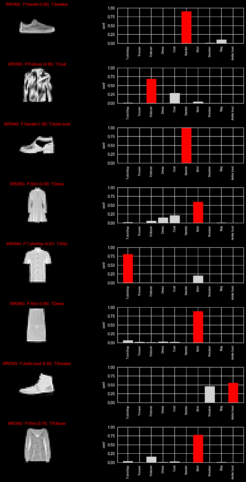
This table generates a view where we can explore the confidence our model had in a prediction: By exploring which weight each class was given, we can see where there was doubt (i.e. multiple classes with a higher weight) versus when the model was certain (only one guess). These examples further confirm our intuition: top-types appear to be more commonly confused by the model. 

Conclusion

And there we have it! We were able to set up and train our first model and already drive some data science insights from our data and model results. Using some of the PyCharm functionalities at this point can speed up the experimentation process by providing access to our documentation and applying code completion directly in the cells. We can even use AI Assistant to help generate some of the graphs we’ll need to further evaluate the TensorFlow model performance and investigate our results.

You can try out this notebook yourself, or better yet, try to generate it with these same tools for a more hands-on learning experience.

Where to go next

This notebook is a minimal, teachable starting point. Here are some practical next steps to try afterwards:

• Replace the dense baseline with a small CNN (Conv2D → MaxPooling → Dense).
• Add dropout or batch normalization to reduce overfitting.
• Apply data augmentation (random shifts/rotations) to improve generalization.
• Use callbacks like EarlyStopping and ModelCheckpoint so training is efficient, and you keep the best weights.
• Export a SavedModel for server use or convert to TensorFlow Lite for edge devices (Raspberry Pi, microcontrollers).

Frequently asked questions

When should I use TensorFlow?

TensorFlow is best used when building machine learning or deep learning models that need to scale, go into production, or run across different environments (cloud, mobile, edge devices). 

TensorFlow is particularly well-suited for large-scale models and neural networks, including scenarios where you need strong deployment support (TensorFlow Serving, TensorFlow Lite). For research prototypes, TensorFlow is viable, but it’s more commonplace to use lightweight frameworks for easier experimentation.

Can TensorFlow run on a GPU?

Yes, TensorFlow can run GPUs and TPUs. Additionally, using a GPU can significantly speed up training, especially for deep learning models with large datasets. The best part is, TensorFlow will automatically use an available GPU if it’s properly configured.

What is loss in TensorFlow?

Loss (otherwise known as loss function) measures how far a model’s predictions are from the actual target values. Loss in TensorFlow is a numerical value representing the distance between predictions and actual target values. A few examples include: 

• MSE (mean squared error), used in regression tasks.
• Cross-entropy loss, often used in classification tasks.

How many epochs should I use?

There’s no set number of epochs to use, as it depends on your dataset and model. Typical approaches cover: 

• Starting with a conservative number (10–50 epochs).
• Monitoring validation loss/accuracy and adjusting based on the results you see.
• Using early stopping to halt training when improvements decrease.

An epoch is one full pass through your training data. Not enough passes through leads to underfitting, and too many can cause overfitting. The sweet spot is where your model generalizes best to unseen data. 

About the author

Iulia Feroli

Iulia’s mission is to make tech exciting, understandable, and accessible to the new generation.

With a background spanning data science, AI, cloud architecture, and open source, she brings a unique perspective on bridging technical depth with approachability.

She’s building her own brand, Back To Engineering, through which she creates a community for tech enthusiasts, engineers, and makers. From YouTube videos on building robots from scratch, to conference talks or keynotes about real, grounded AI, and technical blogs and tutorials – Iulia shares her message worldwide on how to turn complex concepts into tools developers can use every day.

Whether you’re in “fan” or “fear” mode (or somewhere in-between), there’s no denying that Artificial Intelligence changed how we build products, and do business. We’ve always had cybersecurity threats but now the landscape is more complex and we have to consider new forms of fraud detection, customer support, autonomous systems and generative AI hazards.

Plus, as AI capabilities grow, so do the threats targeting them. One of the most critical emerging risk areas is adversarial AI – the use of malicious techniques to exploit, manipulate, and/or compromise AI systems.

Understanding adversarial AI is important for protecting the integrity, reliability, and security of our “AI-powered” products – a phrase we’re all too familiar with. Why? Because, these threats can directly impact business outcomes, leading to financial losses, reputational damage, and the absolute erosion of customer trust, which we’re already seeing.

In this article, we introduce adversarial AI, explore its two primary forms, and outline the main attack surfaces that organizations and software development teams must secure.

The two faces of adversarial AI

Adversarial AI threats generally fall into two broad categories.

1. AI used as a weapon

In the first category, attackers use AI itself to amplify malicious activities. These include:

• Deepfake generation: Creating realistic fake images, videos, or audio to spread misinformation, commit fraud, or damage reputations.
• Automated phishing: Using AI to craft highly personalized phishing emails at scale, increasing success rates while reducing attacker effort.
• AI-generated malware: Developing malware that can identify vulnerabilities and adapt faster than traditional attack techniques.

These attacks aren’t theoretical. They’re already being used to bypass defenses, deceive users, and exploit organizations – often at unprecedented speed and scale. We’ll show you some examples further on but it can be as alarming as it sounds.

2. Attacks targeting AI systems directly

The second category focuses on attacking AI models and systems themselves. These attacks are especially dangerous because they undermine how AI makes decisions, potentially leading to misleading outputs, biased behavior, or unsafe actions.

For organizations relying on AI-driven decisions, compromised models can quietly introduce systemic risk, often without obvious signs until there’s significant damage.

Where attackers focus their efforts

When targeting AI systems, adversaries typically concentrate on three main areas.

1. Attacks on AI algorithms

These attacks target the core learning and decision-making mechanisms of AI systems. By interfering with how models are trained or how they interpret inputs, attackers can influence predictions and outcomes.

This category includes some of the most impactful adversarial techniques, which we explore in detail later in this article.

2. Attacks on generative AI filters

Generative AI systems rely on filters and safeguards to prevent people misusing them – like content moderation filters or information that identifies people personally (email addresses), etc. Attackers exploit weaknesses in these controls using techniques like prompt injection or code injection, helping them get past restrictions.

These filters are applied during input and output and unfortunately provide plenty of opportunity for attackers to get creative to get and use this sensitive information.

When successful, these attacks help adversaries generate harmful content, and/or execute actions that aren’t intended – often leaving the user none the wiser until it’s too late.

3. Supply chain attacks on AI artifacts

AI systems depend a lot on third-party components, including datasets, pre-trained models, APIs, and open-source libraries. Supply chain attacks target these dependencies.

For example, an attacker may compromise an open-source library that’s used during model training or embed malicious code into a dataset. Once it’s already integrated, the compromised component can enable unauthorized access, data exfiltration, or system disruption.

Because these attacks exploit trusted dependencies, they’re especially difficult to detect and can have far-reaching consequences.

Attacks on AI algorithms: real-world examples

Attacks on AI algorithms strike at the foundation of AI systems. When successful, they can cause models to behave incorrectly, unpredictably, or maliciously. Three attack types dominate this category: data poisoning, evasion attacks, and model theft.

Data poisoning attacks

Data poisoning occurs during the training phase of an AI model. Attackers manipulate training data to corrupt the model’s learning process, causing it to internalize false or harmful patterns.

For example, consider a fraud detection model trained to identify suspicious transactions. If an attacker gains access to the training pipeline, they could inject fraudulent transactions labeled as legitimate. As a result, the model becomes less effective at detecting real fraud, exposing the organization to financial risk.

A well-known real-world example is Microsoft’s Tay chatbot, launched in 2016. Tay learned directly from user interactions on Twitter (if you’re a Millennial) or X (If you’re a Gen-Z), and was quickly manipulated into producing offensive and harmful content. This incident highlighted the risks of unmonitored data pipelines and insufficient safeguards during training.

Search engine manipulation offers another example, where poisoned data has been used to surface false information, which breaks user trust in AI-driven systems.

Evasion attacks

Evasion attacks occur after a model has been deployed. Instead of modifying the model, attackers subtly manipulate inputs to cause incorrect predictions.

In fraud detection, this might involve changing spending behavior just enough to avoid triggering alerts, such as breaking large transactions into smaller ones. Each transaction appears legitimate in isolation, allowing fraud to go undetected.

Evasion attacks have also been demonstrated in autonomous driving systems. Researchers have shown that placing small stickers on a stop sign can cause a self-driving car to misinterpret it as a speed limit sign. These changes are often barely noticeable, or even not noticeable at all, to humans but sufficient to confuse the model. This could lead to catastrophic outcomes depending on the different use cases.

Similar techniques can bypass facial recognition systems or other biometric controls, enabling unauthorized access and data theft.

Model theft

Model theft involves stealing or replicating an AI model by repeatedly querying it and analyzing its outputs. Over time, attackers can infer the model’s structure, parameters, or even training data, effectively cloning proprietary intellectual property.

In 2019, researchers demonstrated that a commercial AI model could be replicated with approximately 90% accuracy using only its public interface. By observing how the model responded to carefully chosen inputs, they reconstructed its internal behavior.

A more recent example emerged in 2023 with the Alpaca and OpenLLaMA projects. Attackers queried Meta’s Llama model extensively and analyzed its outputs to reverse-engineer its functionality. This process enabled them to create Alpaca, a model that closely mimicked LLaMA’s performance without direct access to its source code or training data.

Model theft undermines the competitive advantage of proprietary AI systems and enables adversaries to reuse or resell stolen capabilities.

Why this matters for businesses

Data poisoning, evasion attacks, and model theft all compromise the integrity and reliability of AI systems. For businesses, the consequences can include:

• Operational disruptions
• Financial losses
• Intellectual property theft
• Regulatory and compliance risks
• Loss of customer trust

Protecting AI systems requires more than traditional application security. Organizations must design AI with resilience in mind, implementing access controls, monitoring model behavior, validating data pipelines, and securing dependencies throughout the AI supply chain.

What’s next?

Understanding these attack vectors is the first step toward securing AI-powered products. In the next session, we’ll explore attacks on filters in generative AI, where adversaries bypass safeguards to misuse AI capabilities.

By proactively addressing adversarial AI threats, organizations can protect their models, their users, and their business outcomes.

As Qodana continues to develop for a new age of security and quality threats, we’re releasing new features that help protect your codebase so you can focus on quality and debt. Speak to the team to find out how we can help.

Get A Qodana Demo

Introduction

Imagine a user opens your Android app, taps a button, and nothing happens.

The screen freezes.

After a few seconds, Android shows:

Application Not Responding (ANR)

Most users don’t wait.

They close the app and uninstall it.

That’s why ANRs are one of the most dangerous performance issues in Android apps.

According to Android Developers documentation, ANRs happen when the main thread is blocked and cannot respond to user input within a specific time.

And if your ANR rate becomes high, Google Play can reduce your app visibility.

So understanding ANRs is not optional — it’s critical.

**What is an ANR? (Simple Explanation)

Official Definition**

ANR occurs when the UI thread is blocked and cannot process user input or draw frames.

Android shows ANR when:

• Input event not handled within 5 seconds
• BroadcastReceiver runs too long
• Service takes too long to start
• Job or foreground service delays response

Real-World Example

Think of your app like a restaurant.

• UI Thread = Waiter
• Background Thread = Kitchen
• User = Customer

Good Flow

Customer orders → Waiter sends to kitchen → Kitchen prepares → Waiter delivers

Everything runs smoothly.

Bad Flow (ANR)

Customer orders → Waiter goes to kitchen and starts cooking himself

Now:

• No one takes new orders
• No one serves food
• Restaurant stops working

This is exactly what happens when UI thread does heavy work.

Top Causes of ANRs

1. Heavy Work on Main Thread ❌

Problem

Running:

• Network calls
• Database queries
• File reading
• JSON parsing
• Image processing

on UI thread.

Android documentation clearly states:

Keep main thread unblocked and move heavy work to worker threads

2. Long Database or Network Operations ❌

Example:

val data = api.getUsers() // running on main thread

This blocks UI.

Result → ANR.

3. BroadcastReceiver Doing Heavy Work ❌

BroadcastReceiver should do small quick tasks only.

If it runs too long → ANR.

Android recommends moving work to background threads.

4. Service Not Starting in Time ❌

Foreground service must call:

startForeground()

within 5 seconds.

Otherwise → ANR.

5. Deadlocks and Thread Blocking ❌

Example:

Thread A waiting for Thread B
Thread B waiting for Thread A

Result:

App freezes.

Android documentation calls this deadlock, a major ANR cause.

**Common Developer Mistakes

❌ Running API calls in Activity**

override fun onCreate() {
    super.onCreate()

    val users = api.getUsers()
}

Wrong approach.

❌ Large JSON parsing on UI thread

val json = File("data.json").readText()

ANR risk.

Best Practices to Avoid ANRs

✅ Use Coroutines

viewModelScope.launch {
    val users = repository.getUsers()
}

Moves work off main thread.

✅ Use Dispatchers.IO

withContext(Dispatchers.IO) {
    api.getUsers()
}

Optimized for I/O.

✅ Use Flow for Continuous Data

repository.getUsersFlow()
    .flowOn(Dispatchers.IO)

Efficient and non-blocking.

✅ Use WorkManager for Background Tasks

Good for:

• Sync
• Upload
• Downloads
• Scheduling

✅ Keep BroadcastReceiver Lightweight

override fun onReceive(context: Context, intent: Intent) {

    CoroutineScope(Dispatchers.IO).launch {
        repository.sync()
    }
}

Modern Kotlin Code Example
Repository

class UserRepository(
    private val api: UserApi
) {

    suspend fun getUsers(): List<User> {
        return withContext(Dispatchers.IO) {
            api.getUsers()
        }
    }
}

ViewModel

@HiltViewModel
class UserViewModel @Inject constructor(
    private val repository: UserRepository
) : ViewModel() {

    private val _users = MutableStateFlow<List<User>>(emptyList())
    val users = _users.asStateFlow()

    init {
        loadUsers()
    }

    private fun loadUsers() {
        viewModelScope.launch {
            _users.value = repository.getUsers()
        }
    }
}

Jetpack Compose UI

@Composable
fun UserScreen(viewModel: UserViewModel) {

    val users by viewModel.users.collectAsState()

    LazyColumn {
        items(users) { user ->
            Text(user.name)
        }
    }
}

Real-World Use Case
Video Fetching App

Scenario:

App scans device videos.

Wrong

Scanning files in Activity.

UI freezes.

ANR occurs.

Correct

• Splash loads videos
• Repository uses Dispatchers.IO
• Flow emits data
• UI updates smoothly

Result:

✔ No ANR
✔ Smooth scrolling
✔ Fast loading
✔ Better Play Store rating

**Key Takeaways

Core Rule**

Never block the main thread

Important Points

✔ UI thread must always be free
✔ Move heavy work to background threads
✔ Use Coroutines and Flow
✔ Keep BroadcastReceiver lightweight
✔ Use WorkManager for long tasks
✔ Avoid deadlocks and thread blocking
✔ Monitor ANR in Play Console

Conclusion

ANRs are not just performance issues.

They directly impact:

• User experience
• App rating
• Play Store ranking
• Revenue

The safest strategy is simple:

Keep the UI thread clean and move all heavy work to background threads.

If you follow Android’s official guidelines and modern Kotlin practices, ANRs can be almost eliminated.

Feel free to reach out to me with any questions or opportunities at (aahsanaahmed26@gmail.com)
LinkedIn (https://www.linkedin.com/in/ahsan-ahmed-39544b246/)
Facebook (https://www.facebook.com/profile.php?id=100083917520174).
YouTube (https://www.youtube.com/@mobileappdevelopment4343)
Instagram (https://www.instagram.com/ahsanahmed_03/)

Let me start with a confession. For years, I treated geospatial data like a messy closet—shove everything in, slam the door, and pray nobody asks for a “nearby” anything. Then came the project that broke me: a real-time delivery tracker with 50k points and a naive WHERE sqrt((x1-x2)^2 + (y1-y2)^2) < 0.01 query that took forty-five seconds. My CTO’s Slack message just said: “Oof.”

That night, I discovered PostGIS. And I learned that working with space on a computer isn’t just math—it’s an art form. One where you’re both the cartographer and the gallery curator.

So grab coffee. Let me walk you through the journey from “it works on my laptop” to “this scales like a dream.” No marketing fluff. Just the battle scars and the beautiful abstractions that saved my sanity.

Act I: The Naive Cartographer (or, Why Euclidean Distance Lies)

You know the scene. You have a restaurants table with lat and lon as plain decimals. A user wants all taco joints within 1 km. Your first instinct:

SELECT * FROM restaurants
WHERE sqrt((lat - 40.7128)^2 + (lon - -74.0060)^2) < 0.009;  -- ~1km in deg?!

This is wrong on two levels. First, degrees are not kilometers—unless you enjoy eating polar-bear tacos at the equator. Second, that query will do a full table scan every time. Your database is now screaming like a dying server fan.

The awakening: PostGIS introduces geometry types and a proper spatial relationship model. The same query becomes:

SELECT * FROM restaurants
WHERE ST_DWithin(
  geom, 
  ST_SetSRID(ST_MakePoint(-74.0060, 40.7128), 4326),
  1000  -- meters, thank you very much
);

But wait—that still scanned everything? Right. Because we forgot the most important part.

Act II: The Index as a Legend (GIST is Your Compass)

Here’s where the art begins. A normal B-tree index is like alphabetizing a bookshelf—great for “title = X”. But spatial data is a map. You don’t search a map by flipping pages; you fold it, you zoom, you glance at regions.

Enter GIST (Generalized Search Tree). Think of it as an origami master that folds your 2D (or 3D, or 4D) space into a tree of bounding boxes. When you query “find points within 1 km,” PostGIS uses the index to discard entire continents of data instantly.

Create it:

CREATE INDEX idx_restaurants_geom ON restaurants USING GIST (geom);

That one line turned my 45-second query into 80 milliseconds. I literally laughed out loud. My cat left the room.

But indexing isn’t magic—it’s a trade-off. GIST indexes are slightly slower to update (insert/update/delete) than B-trees. For a write-heavy geospatial table, you’ll need to tune autovacuum or batch your writes. More on that later.

Art lesson: A GIST index is like the legend on a map—it doesn’t show every tree, but it tells you exactly how to find the forest.

Act III: The Palette of Spatial Functions (Don’t Paint with a Hammer)

PostGIS has hundreds of functions. You only need a dozen to be dangerous. Here’s my everyday toolkit, refined through actual pain:

Real example: Find the 10 closest coffee shops to a user, within 5 km, ordered by distance.

SELECT name, ST_Distance(geom, user_geom) AS dist
FROM coffee_shops
WHERE ST_DWithin(geom, user_geom, 5000)
ORDER BY geom <-> user_geom
LIMIT 10;

That <-> operator? It’s the KNN (K-Nearest Neighbor) index-assisted magic. Without it, PostGIS would calculate distance for every shop within 5 km, then sort. With it, the index walks the tree and returns candidates in approximate order. It’s not exact until the final sort, but it’s blindingly fast.

Act IV: The Geometry vs. Geography Schism (A Tale of Two Earths)

You’ll hit this around 2 AM. Your polygons on a city scale work fine. Then you try to calculate the area of a country and get numbers that would make a flat-earther nod approvingly.

Geometry: Treats the Earth as a flat Cartesian plane. Good for local projects (a few hundred km). Fast. Simple. Wrong for global distances.

Geography: Uses a spheroidal model (WGS84 by default). Accurate for distance, area, and bearing across the globe. Slower, because it’s doing real math.

My rule of thumb:

• Store as geometry with SRID 4326 (lat/lon coordinates). It’s lightweight.
• Use geography casting when you need Earth-aware calculations: geom::geography.
• Index both – but a GIST on geography is larger and slightly slower.

Pro tip: For large tables with global queries, add a geog column as geography(Point, 4326) and index that. Then you can write clean queries like:

SELECT * FROM sensors
WHERE ST_DWithin(geog, ST_MakePoint(lon, lat)::geography, 50000); -- 50 km

No casting in the query means the index gets used without hesitation.

Act V: The Performance Trap (What They Don’t Put in the Brochure)

You’ve indexed everything. Queries are snappy. Then you deploy to production and… it’s slow again. Why?

Three silent killers:

1. Implicit casting in the WHERE clause

   WHERE ST_DWithin(geom::geography, ...) – the cast happens before the index lookup. PostGIS can’t use a GIST on geometry for a geography query. Keep types consistent.

2. Using ST_Distance for filtering

   -- This is a full scan. Always.
   WHERE ST_Distance(geom, point) < 1000

ST_DWithin exists for a reason. Use it.

1. Over-indexing on large polygons
   A GIST index on a column full of complex polygons (e.g., country borders) can be huge. Consider storing a simplified “envelope” geometry for coarse filtering, then refine with exact ST_Intersects.

Real story: We had a table of 2M GPS traces. Queries were fast in dev (10k rows). In prod, EXPLAIN ANALYZE showed a bitmap heap scan—PostGIS was reading half the table anyway. Why? The distribution was clustered, but our random test data wasn’t. We added CLUSTER idx_restaurants_geom ON restaurants to physically reorder rows by spatial locality. Query time dropped from 4 seconds to 200ms.

Act VI: The Artistic Workflow (How to Think Spatially)

After two years of wrestling with PostGIS, I’ve developed a kind of intuition. It’s like learning to see negative space in a drawing. Here’s my mental checklist before writing any spatial query:

1. Draw it first – I keep a whiteboard or a quick QGIS window. Visualizing bounding boxes and intersections saves hours.
2. Start with the index – Write the query assuming the index will do the heavy lifting. Filter early, refine late.
3. Test with a point – Run EXPLAIN (ANALYZE, BUFFERS) on a single coordinate. Look for “Seq Scan” – if you see it, your index isn’t being used.
4. Think in meters, store in degrees – Use geography for distances, geometry for operations. Cast explicitly.
5. Batch your writes – A GIST index rebuild on 1M rows takes minutes. Do it nightly, not per insert.

Epilogue: You Are Now a Spatial Artist

PostGIS isn’t just a library. It’s a lens that changes how you see data. Suddenly every “near me” button, every delivery route, every heatmap becomes a solvable puzzle instead of a performance nightmare.

The journey from sqrt(lat^2 + lon^2) to elegant ST_DWithin with a GIST index is the difference between a child’s crayon scribble and a Monet. You’ve learned the brushstrokes. Now go paint some maps.

And when someone asks you, “Can you find all points within a polygon?” – smile, open your terminal, and whisper: “Watch this.”

This is a follow-up to Mandelbrot Set in JS – Zoom In.
In that article we built a Mandelbrot renderer using Canvas and Web Workers, with click-to-zoom.
This post covers what broke after ~16 zooms, why it broke (floating-point precision),
and how we replaced click zoom with a smooth scroll-based zoom that also lets you zoom back out.

The Problem: Everything Turns Black After ~16 Clicks

If you played with the previous demo long enough, you noticed something strange: after zooming in about 16 times, the fractal starts looking pixelated, blocky, and eventually the entire canvas turns solid black.

This isn’t a bug in the Mandelbrot math. The set is infinitely detailed, there’s always more structure to see. The problem is in how computers store decimal numbers.

Root Cause: JavaScript Numbers Have Limited Precision

JavaScript (like most languages) stores all numbers as 64-bit IEEE 754 doubles. This is just the standard format computers use for decimal numbers, and it gives you about 15 to 17 significant digits of precision. That sounds like a lot, but zoom burns through those digits very fast.

How the old zoom worked

Each click zoomed to a window of 2 × ZOOM_FACTOR × canvas_width pixels centered on the click point. With ZOOM_FACTOR = 0.1, each zoom reduced the visible range to 20% of the previous range:

const zfw = WIDTH * ZOOM_FACTOR;  // 800 * 0.1 = 80px on each side
REAL_SET = {
  start: getRelativePoint(e.pageX - canvas.offsetLeft - zfw, WIDTH, REAL_SET),
  end:   getRelativePoint(e.pageX - canvas.offsetLeft + zfw, WIDTH, REAL_SET),
};

The coordinate range after N clicks shrinks like this:

range_after_N = initial_range × 0.2^N

At click 15, the range is 7.5e-12. If your center is around -0.7, the coordinates look like:

start: -0.700000000003750
end:   -0.700000000003751

Those two numbers share 15 digits. With only 15 to 17 digits of total precision, the difference between adjacent pixels becomes too small to represent. Every pixel ends up mapping to the same value. Result: a grid of identical colors, pixelation, black.

This is called catastrophic cancellation: when you subtract two numbers that are almost the same, you lose all the useful digits.

The Fix, Part 1: Replace Click with Scroll Zoom

The first change is switching from click to wheel (scroll). This gives us:

• Zoom in (scroll up) and zoom out (scroll down) with the same gesture
• Smooth, step-by-step control over the zoom level
• The zoom always centers on the cursor position

Here is the complete new listener:

const ZOOM_FACTOR = 0.8; // each scroll step = 80% of current range (zoom in)
const MIN_RANGE = 1e-12; // safety limit, stop before precision breaks down

const startListeners = () => {
  canvas.addEventListener('wheel', (e) => {
    e.preventDefault();
    const zoomIn = e.deltaY < 0;
    const factor = zoomIn ? ZOOM_FACTOR : 1 / ZOOM_FACTOR;

    const realRange = REAL_SET.end - REAL_SET.start;
    const imagRange = IMAGINARY_SET.end - IMAGINARY_SET.start;
    const newRealRange = realRange * factor;
    const newImagRange = imagRange * factor;

    // Stop zooming in before precision collapses
    if (newRealRange < MIN_RANGE || newImagRange < MIN_RANGE) return;

    // Map cursor pixel to a point in the complex plane
    const mouseX = e.pageX - canvas.offsetLeft;
    const mouseY = e.pageY - canvas.offsetTop;
    const centerReal = getRelativePoint(mouseX, WIDTH, REAL_SET);
    const centerImag = getRelativePoint(mouseY, HEIGHT, IMAGINARY_SET);

    REAL_SET = {
      start: centerReal - newRealRange / 2,
      end:   centerReal + newRealRange / 2,
    };
    IMAGINARY_SET = {
      start: centerImag - newImagRange / 2,
      end:   centerImag + newImagRange / 2,
    };

    Mandelbrot();
  }, { passive: false }); // passive: false is required to call e.preventDefault()
};

Let’s go through each decision:

e.preventDefault() + { passive: false }

By default, browsers treat wheel events as passive for performance, assuming you won’t stop the default scroll behavior. We need to prevent the page from scrolling while the user zooms the fractal, so we have to opt out. Without { passive: false }, calling preventDefault() does nothing and the page scrolls anyway.

factor = zoomIn ? ZOOM_FACTOR : 1 / ZOOM_FACTOR

Zooming in multiplies the range by 0.8 (makes it smaller). Zooming out divides by 0.8 (makes it bigger). This keeps zoom in and out symmetric, so ten zooms in followed by ten zooms out brings you back to exactly where you started.

Centering on the cursor

The new approach maps the cursor pixel to a point in the complex plane, then builds the new window symmetrically around it:

const centerReal = getRelativePoint(mouseX, WIDTH, REAL_SET);
const centerImag = getRelativePoint(mouseY, HEIGHT, IMAGINARY_SET);

getRelativePoint converts a pixel position to a coordinate using a simple formula:

const getRelativePoint = (pixel, length, set) =>
  set.start + (pixel / length) * (set.end - set.start);

ZOOM_FACTOR = 0.8 instead of 0.1

With 0.1, each click zoomed to 20% of the range, which was very aggressive. The precision limit was hit in 16 steps. With 0.8, each scroll step reduces the range by only 20%, so you can zoom about 130 times before hitting the same limit. It also feels much smoother to use.

The Fix, Part 2: The Precision Guard

if (newRealRange < MIN_RANGE || newImagRange < MIN_RANGE) return;

With MIN_RANGE = 1e-12 we stop zooming in when the coordinate window gets too small. At that scale, the numbers don’t have enough precision left to render a meaningful image. Instead of turning black, the fractal just stays frozen at the last good zoom level. The scroll event is silently ignored.

How the Renderer Still Works

For context, here is how each column of pixels is computed in the Web Worker. This part is the same as in the previous article:

// worker.ts, runs in a separate thread via Vite's ?worker import

const MAX_ITERATION = 1000;

function mandelbrot(c: { x: number; y: number }): [number, boolean] {
  let z = { x: 0, y: 0 };
  let n = 0;
  let d = 0;
  do {
    const p = {
      x: Math.pow(z.x, 2) - Math.pow(z.y, 2),
      y: 2 * z.x * z.y,
    };
    z = { x: p.x + c.x, y: p.y + c.y };
    d = 0.5 * (Math.pow(z.x, 2) + Math.pow(z.y, 2));
    n += 1;
  } while (d <= 2 && n < MAX_ITERATION);
  return [n, d <= 2];
}

This is the core iteration: z → z² + c. A point c is in the Mandelbrot set if |z| never escapes 2 after MAX_ITERATION steps. Points that do escape get colored by how fast they did it (the value of n).

The main thread sends one message per column and the worker replies with the results:

// columns are dispatched in random order for a cool reveal effect
const launchTasks = () => {
  while (TASKS.length > 0) {
    const [col] = TASKS.splice(Math.floor(Math.random() * TASKS.length), 1);
    worker.postMessage({ col });
  }
};

Current Limitations

Here is an honest list of what this implementation still can’t do:

Future Improvements

1. Arbitrary Precision with decimal.js

To zoom beyond ~130 steps you need more than the standard 64-bit number format. The decimal.js library lets you set how many digits of precision you want:

import Decimal from 'decimal.js';

Decimal.set({ precision: 50 }); // 50 significant digits

const newRange = new Decimal(realRange).mul(factor);
const center  = new Decimal(realSet.start)
  .plus(new Decimal(mouseX).div(WIDTH).mul(new Decimal(realSet.end).minus(realSet.start)));

The downside is that this kind of math is 10 to 100 times slower than normal numbers, so you would need to lower the canvas resolution or the number of iterations to keep things running at a good speed.

2. Perturbation Theory

This is the technique used by professional deep-zoom renderers like Kalles Fraktaler. The idea is to compute one very precise reference point and then calculate all other pixels as small adjustments relative to that point, using regular numbers. This can reach zoom depths of 10^1000 and beyond, with good performance, but it requires a solid math background to implement.

3. Adaptive MAX_ITERATION

Instead of a fixed limit, scale the number of iterations based on how deep the zoom is, so shallow views are fast and deep views show more detail:

const maxIter = Math.floor(100 + zoomLevel * 50);

4. RAF Throttle

The scroll event fires much faster than the renderer can keep up. Using requestAnimationFrame would skip frames that come in too quickly and only render when the browser is ready:

let rafId: number;
canvas.addEventListener('wheel', (e) => {
  e.preventDefault();
  updateCoordinates(e);
  cancelAnimationFrame(rafId);
  rafId = requestAnimationFrame(() => Mandelbrot());
}, { passive: false });

5. Pinch-to-Zoom (Mobile)

Handle touchstart and touchmove with two fingers to calculate a scale factor and apply the same zoom logic.

Summary of Changes

Try It Live

You can see the demo running on quijosakaf.com and find the full source on GitHub.

Repository:
github

If you want to experiment, try changing ZOOM_FACTOR between 0.5 (aggressive) and 0.95 (very smooth). The math works the same either way, it’s just a personal preference.

Thanks for Reading

If you made it this far, thank you so much. This kind of topic can get complicated fast, and I appreciate you sticking with it.

I want to be honest: this post was written with the help of AI (Claude). Concepts like IEEE 754, catastrophic cancellation, arbitrary precision arithmetic, and perturbation theory were things I did not know about before I started digging into why the zoom was breaking. The AI helped me understand why each thing was happening and gave me the right words to describe it, which made it much easier to explain here.

The demo will keep improving. The improvements listed above (RAF throttling, adaptive iterations, arbitrary precision, pinch-to-zoom) are real next steps I plan to work on. If you have ideas, found a bug, or just want to talk about fractals, drop a comment below.